We presented the work we did on 3Di at the IEMSS conference. You can find both the presentation and the paper online.
Videos
I used the following videos in the presentation.
Other presentations from Deltares include:
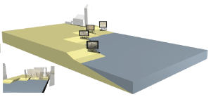
In the night of June 11, 1962 three inmates escaped from Alcatraz.
Here are some visualizations of the escape. This is work in progress. The model and visualizations are created together with Olivier Hoes, Martijn Siemerink and Gena Donchyts.
Created with 3Di, python-subgrid, matplotlib, VTK, cloudmade.
An overview
These are some notebooks and the material used by the Python for Engineers course.
This is the lunch lecture that I gave at the L&R faculty.
One of the questions that came up was what the preferred way is to install python on OSX. This was related to some recent problems that people had with the latest version of OSX. Some of the issues that you can run into while installing extra packages are a missing png library issue and missing compilers .
Some of the options you have under OSX are, in my personal order of preference:
- Install macports. Then install matplotlib sudo port install py27-matplotlib.
- Install homebrew. Then install python, then matplotlib using pip pip install matplotlib.
- Get the enthought python distribution (now called Canopy).
- Get the continuum distribution.
You probably don't want to use the python version that comes preinstalled with OSX. Using one of the other options keeps your python environment separate from your system environment and you'll have a more recent python version.
You can also use virtualenv to use multiple different python environments.
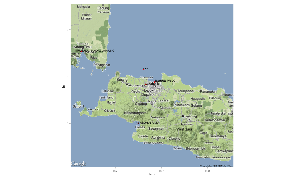
This is an example of how to use the sealevel R package. This package is part of OpenEarth and available through r-forge for the convenience of R users. See Trends in Sea-Level Trend Analysis for a discussion on sea-level trend analysis.
This example generates an overview of tide gauges near Jakarta and generates a plot of the measurements of the nearby stations.
|

|
# This is an example of how to get tide gauge data for Jakarta

library(sealevel) # the sealevel package
library(plyr) # reshape
library(ggplot2) # grammar of graphics
library(ggmap) # plot on top of googlemap

# get all the tide gauge data from PSMSL

# For Jakarta no revised local reference data is available.
# Please see the PSMSL site for details

# Get the url for the metric dataset
url <- get.psmsl.url(type='metric')

# Get the name of the file
path <- basename(url)
# Download all data (takes a while)
download.file(url, path)

# Read all monthly data
stations <- read.psmsl(path)

# Create an overview of all locations and names
stations.latlon <- ldply(stations, function(station){data.frame(lat=station$lat, lon=station$lon, name=station$name)})

# Plot a map of Jakarta
# 6.2S 106.8E
jakarta <- get_map(location = c(lon = 106.8, lat = -6.2), zoom = 8)
jakarta.map <- ggmap(jakarta)
# Plot the nearby tide gauges with the name as a lable
p <- jakarta.map + geom_point(data=stations.latlon, aes(x=lon, y=lat), color='red')  + geom_text(data=stations.latlon, aes(x=lon, y=lat, label=name), hjust=0.1, vjust=0.1, size=3)

# Save it to png
png('tidegaugemapjakarta.png', width=1000, height=600)
print(p)
dev.off()

# compute the distance from jakarta
dist <-  laply(stations, function(station){sqrt((station$lon - 106.8)**2 + (station$lat - -6.2)**2)})
# use the first 5 stations
jakarta.stations <- stations[order(dist)][1:10]
# combine them into 1 data fram
jakarta.df <- ldply(jakarta.stations, function(station) {df <- station$data; df$name <- station$name; df$waterlevel <- df$waterlevel - mean(df$waterlevel, na.rm=TRUE); return(df)})
# categorize by name
jakarta.df$name <- factor(jakarta.df$name)
# plot all gauges in one plot
jakarta.df$waterlevel <- jakarta.df$waterlevel + 100*as.numeric(jakarta.df$name)
p <- ggplot(jakarta.df, aes(year.month,waterlevel, color=name)) + geom_line() + geom_smooth() + labs(x='year', y='water level [mm]')

# Save it to png
png('tidejakarta.png', width=1000, height=600)
print(p)
dev.off()
I just made the sealevel R package, which we used for the sea-level rise articles, available. It provides some functions to quickly download, read and analyse the global tide gauges and satellite data.
All suggestions, patches, comments are welcome. This package is part of OpenEarth but available through r-forge for the convenience of R users.
- Trends in Sea-Level Trend Analysis
- The Effect of the 18.6-Year Lunar Nodal Cycle on Regional Sea-Level Rise Estimates
Example
The code below generates the plot of the Dutch tide gauges.
# install.packages("sealevel", repos="http://r-forge.r-project.org")
library(sealevel)
library(ggplot2)
library(plyr)

# Load the Dutch sealevel data
data(dutch)

# Let's plot them all

# The stations are a list of objects, but we can make a data frame like this
station2df <- function(x){
  df <- x$data
  df$name <- x$name
  # set -999 to missing
  df$waterlevel[df$waterlevel==-999.9] <- NA
  return(df)
}

# Let's do bit of map reducing, list -> station2df -> data.frame
dutchdf <- ldply(dutch, station2df)
# Now make a factor instead from the strings
dutchdf$name <- as.factor(dutchdf$name)
# so we can use it to shift the waterlevels a bit
dutchdf$waterlevel <- dutchdf$waterlevel - as.numeric(dutchdf$name)*10

# Use the gramar of graphics approach
p <- ggplot(dutchdf, aes(year, waterlevel, color=name))
# Fit a nodal cycle (long term tide), See Baart et al 2012 in JCR.
p + geom_point() + geom_smooth(method='lm', formula=y~x+I(cos(2*pi*x/18.613))+I(sin(2*pi*x/18.613)))
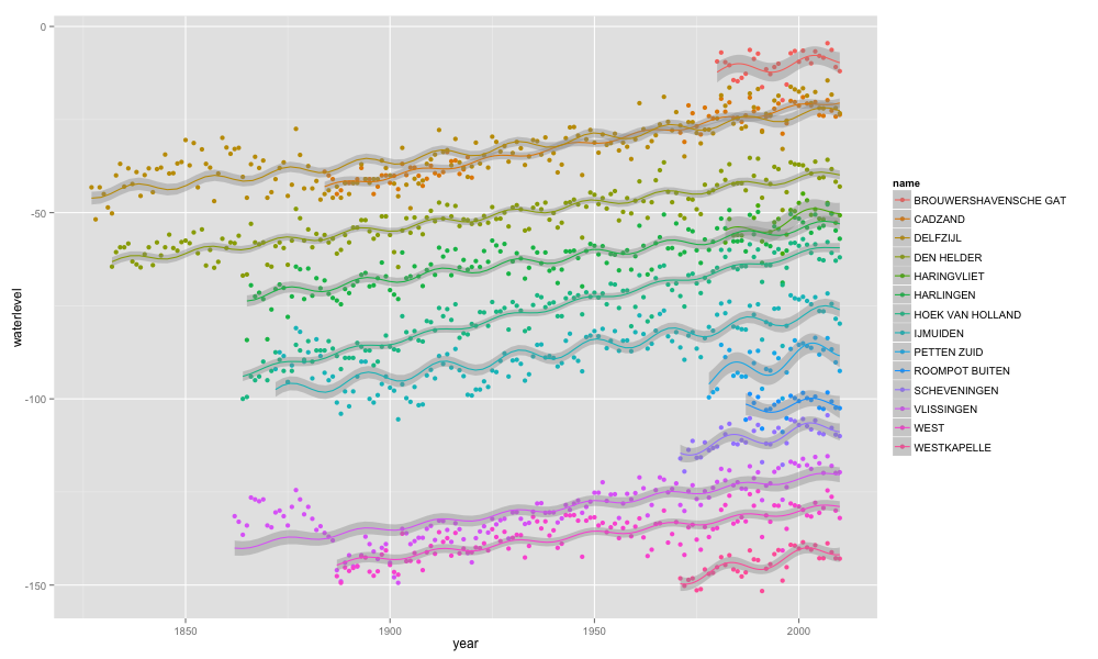
Notice that after the last 6 years of (average) sea-level decline we are about to see a rising sea level at the Dutch coast again for the next 12 years.
This presentation was given at the Deltares statistics community lunch lecture. It discusses some best and worst practices in estimating sea-level rise. The presentation is based on two articles:
At the EGU, in the session about aeolian transport , we presented the integrated coastal model.
Please find the EGU Aeolian transport presentation in the attachments.
More info can be found here:
Sourcecode: http://oss.deltares.nl (under xbeach, info on compiling)
Dune: http://www.comphys.ethz.ch/hans/dunes.html
If you want to compile the coupled version of Dune and XBeach under windows you need the following.
- Cygwin (including gfortran, gcc, libtool, automake, libfftw3-devel, libfftw3)
- MPICH2 source code release
- netcdf>=4.1 source code
- The following XBeach branches:
- trunk
- branches/esmf
- branches/dune/Muller
- branches/XD_XB_coupling
You can follow these steps:
- Install cygwin
- Compile MPICH2 using gfortran and make install (check if mpif90 is available)
- Compile netCDF using gfortran and make install (check if nc-config is available)
- Compile XBeach (--with-netcdf --without-mpi, mpi is not supported yet ), should generate a file called libxbeach.la
- Compile dune in branches/dune/Muller (should generate a file called libdune.la)
- Compile esmf (use settings like in settings under condition wl01485) (should generate a file called esmf.mod)
- Compile XD_XB_Coupling (double check the Makefile.am, to see if it uses the correct locations for the libraries that were made in the previous steps). (should generate a file called xdunexbeach)
Setting up a simulation:
- Create a directory with both dune and xbeach input (default.par, data/, params.txt)
- Create a coupler setup file (see examples in coupler directory)
- run xdunexbeach from the current directory.
Debugging:
Run the command path/to/xdunexbeachdir/libtool --mode=execute gdb path/to/xdunexbeachdir/xdunexbeach.
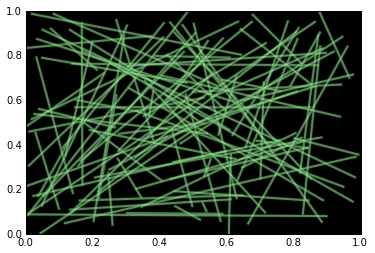
If you want to give your plots a bit of a high tech look you can use a green phosphor style.
Let's try and create some illuminated storm tracks. The basic technique is to draw a line with a glow around it. This can be done by plotting transparent lines on top of each other. Below you see the basic glow effect. It is a bit exaggerated but it still looks ok.
# Set the background color to black for some illumination effects
rcParams['axes.facecolor'] = 'black'
# Define a new figure
f = figure() # figsize=(15,10))
# Add a subplot (so we can add plots to an axes)
ax = f.add_subplot(1,1,1)
for i in range(10):
    # define random points
    x = random.rand(2)
    y = random.rand(2)
    # Now create 3 lines on top of each other
    ax.plot(x,y, 'g-', linewidth=40, alpha=0.2)
    ax.plot(x,y, 'g-', linewidth=30, alpha=0.2)
    ax.plot(x,y, 'w-', linewidth=20, alpha=0.4)

Now make the lines a bit smaller.
# Define a new figure
f = figure() # figsize=(15,10))
# Add a subplot (so we can add plots to an axes)
ax = f.add_subplot(1,1,1)
for i in range(100):
    # define random points
    x = random.rand(2)
    y = random.rand(2)
    # Now create 3 lines on top of each other
    ax.plot(x,y, 'g-', linewidth=4, alpha=0.2)
    ax.plot(x,y, 'g-', linewidth=3, alpha=0.2)
    ax.plot(x,y, 'w-', linewidth=2, alpha=0.4)
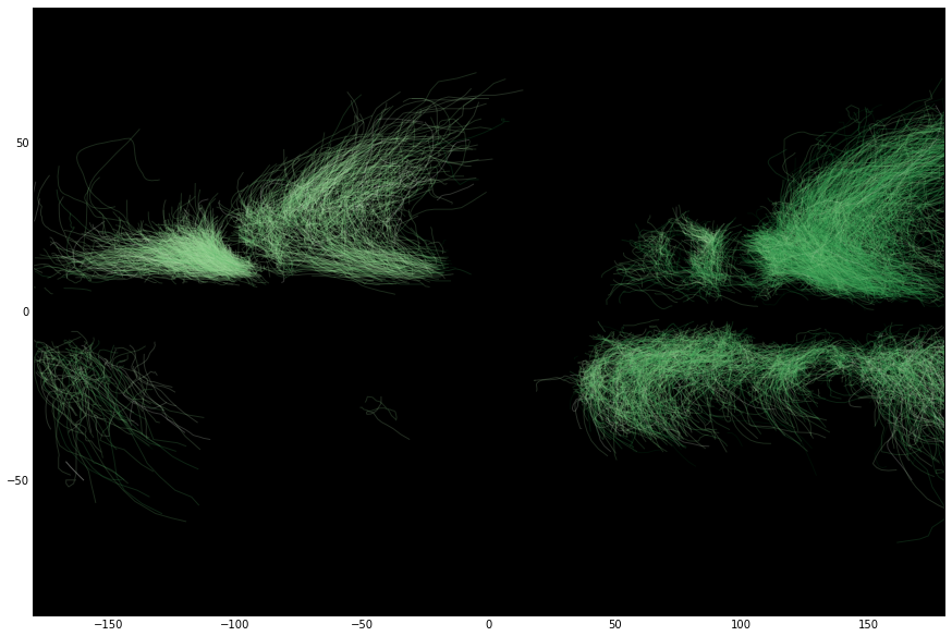
When you create more than about 1000 lines there's no need to add the background lines anymore.
I got the dataset from NOAA
import os
import netCDF4

from matplotlib.collections import LineCollection
from matplotlib.cm import ScalarMappable
import numpy as np

datadir = '/Users/fedorbaart/Downloads/ibtracs'
filenames = os.listdir(datadir)


# Define a new figure
f = figure(figsize=(15,10))
# Add a subplot (so we can add plots to an axes)
ax = f.add_subplot(1,1,1)

# Create a normalization function to scale the color from green to white
# not sure what the max of windspeed is
norm = matplotlib.colors.Normalize(0,40)
# use only 1000 files (there's 15000 of them)
for filename in filenames[-5000:]:
    if not filename.endswith('.nc'):
        continue
    ds = netCDF4.Dataset(os.path.join(datadir, filename))
    # Copy the arrays
    lat = ds.variables['lat_for_mapping'][:]
    lon = ds.variables['lon_for_mapping'][:]
    wind = ds.variables['wind_for_mapping'][:]
    # close the file
    ds.close()

    # Now just create 1 line because we have too much green otherwise...
    linecol = LineCollection((np.c_[lon, lat],),
                             linestyle='solid', cmap=matplotlib.cm.Greens_r,
                             alpha=0.2)
    # Use 1 as a linewidth (I think this is in pixels
    linecol.set_linewidth(1)
    # Use the normalized windspeed
    linecol.set_array(norm(wind))
    # The normalized windspeed has range 0-1
    linecol.set_clim(0,1.0)

    ax.add_collection(linecol)
# Reset the limits on the axis, after each plot
ax.set_xlim(-180,180)
# For y also
ax.set_ylim(-90,90)
Calling fortran from the outside world. Using iso_c_bindings this is a bit easier. Here you can find some fortran examples and see how you can call these functions from python using ctypes and numpy.
The fortran code.
module test
use iso_c_binding
implicit none
integer, parameter :: MAXSTRLEN = 512
contains

! Utility functions
! fortran character(len=*) are not compatible with c
! To be compatible with c, strings sould be copied to a c_char array
function char_array_to_string(char_array, length)
  integer(c_int) :: length
  character(c_char) :: char_array(length)
  character(len=length) :: char_array_to_string
  integer :: i
  do i = 1, length
     char_array_to_string(i:i) = char_array(i)
  enddo
end function char_array_to_string

! C ends strings with a \0 character. Add this so it is received correctly in c compatible languages
function string_to_char_array(s, length)
  integer(c_int) :: length
  character :: s(*)
  character(c_char) :: string_to_char_array(length)
  integer :: i
  do i = 1, length
     string_to_char_array(i:i) = s(i)
  enddo
  string_to_char_array(i+1:i+1) = C_NULL_CHAR
end function string_to_char_array


! 1 int
integer(c_int) function oneint(arg1) bind(C, name="oneint")
  integer(c_int), intent(inout) :: arg1
  arg1 = 111
  oneint = 123
end function oneint

! 1 double
integer(c_int) function onedouble(arg1) bind(C, name="onedouble")
  real(c_double), intent(inout) :: arg1
  arg1 = 1.11d0
  onedouble = 123
end function onedouble


! 10by10 double
integer(c_int) function twobytwodouble(x) bind(C, name="twobytwodouble")
  real(c_double),intent(inout)  :: x(2,2)
  x = 4
  x(2,1) = 21
  x(1,2) = 12
  twobytwodouble = 123
end function twobytwodouble


! 10by10 double
integer(c_int) function twobythreedouble(x) bind(C, name="twobythreedouble")
  real(c_double),intent(inout)  :: x(2,3)
  x = 6
  x(2,1) = 21
  x(1,3) = 13
  twobythreedouble = 123
end function twobythreedouble

integer(c_int) function twobytwodoublepointer(ptr) bind(C, name="twobytwodoublepointer")
  type(c_ptr), intent(inout) :: ptr
  real(c_double), target, save  :: x(2,2)

  x = 4
  x(2,1) = 21
  x(1,2) = 12
  ptr=c_loc(x)
  twobytwodoublepointer = 123
end function twobytwodoublepointer


! 10by10 double pointer
integer(c_int) function twobythreedoublepointer(ptr) bind(C, name="twobythreedoublepointer")
  type(c_ptr), intent(inout) :: ptr
  ! Save is required here for the memory to remain available after the function call
  real(c_double), target, save  :: x(2,3)
  x = 6
  x(2,1) = 21
  x(1,3) = 13
  ptr = c_loc(x)
  twobythreedoublepointer = 123
end function twobythreedoublepointer

! character
integer(c_int) function letter(arg1) bind(C, name="letter")
  character(kind=c_char), intent(inout) :: arg1
  arg1 = 'W'
  letter = 123
end function letter

! string in (string in length is not fixed but internally you need to set a fixed string length)
integer(c_int) function stringin(arg1) bind(C, name="stringin")
  character(kind=c_char), intent(in) :: arg1(*)
  character(len=MAXSTRLEN) :: string
  string = char_array_to_string(arg1, MAXSTRLEN)
  write(*,*)string
  stringin = 123
end function stringin

! string out (requires fixed number of letters)
integer(c_int) function stringout(arg1) bind(C, name="stringout")
  ! Output string has to be fixed
  character(kind=c_char), intent(out) :: arg1(MAXSTRLEN)
  character(len=MAXSTRLEN) :: string
  string = "Hello from fortran"
  arg1 = string_to_char_array(string, len(trim(string)))
  stringout = 123
end function stringout


end module test
The corresponding python code.
#!/usr/bin/env python
import numpy as np
from ctypes import (CDLL, POINTER, ARRAY, c_void_p,
                    c_int, byref,c_double, c_char,
                    c_char_p, create_string_buffer)
from numpy.ctypeslib import ndpointer
import os

dllpath = os.path.abspath("test.dylib") # or .dll or .so
libtest = CDLL(dllpath)

# Define some extra types
# pointer to a double
c_double_p = POINTER(c_double)
# pointer to a integer
c_int_p = POINTER(c_int)

shape2x2=(2,2)
# Pointer to a 2x2 double in fortran layout
c_double2x2_c = ndpointer(shape=shape2x2, dtype="double", flags="C")
c_double2x2_f = ndpointer(shape=shape2x2, dtype="double", flags="FORTRAN")
# Pointer to a pointer to a 10x10 double in fortran layout
c_double2x2_f_p = POINTER(c_double2x2_f)
c_double2x2_c_p = POINTER(c_double2x2_c)
shape3x2=(3,2)
shape2x3=(2,3)
# Pointer to a 2x3,3x2 double in fortran layout
c_double2x3_c = ndpointer(shape=shape2x3, dtype="double", flags="C")
c_double2x3_f = ndpointer(shape=shape2x3, dtype="double", flags="FORTRAN")
c_double3x2_c = ndpointer(shape=shape3x2, dtype="double", flags="C")
c_double3x2_f = ndpointer(shape=shape3x2, dtype="double", flags="FORTRAN")
# Pointer to a pointer to a 2x3,3x2 double in fortran layout
c_double2x3_f_p = POINTER(c_double2x3_f)
c_double2x3_c_p = POINTER(c_double2x3_c)
c_double3x2_f_p = POINTER(c_double3x2_f)
c_double3x2_c_p = POINTER(c_double3x2_c)

# Pointer to a character pointer
c_char_p_p = POINTER(c_char_p)
MAXSTRLEN=512
# Character array (Fortran can only return c_char arrays in c compatible mode)
c_char_array = ARRAY(c_char,MAXSTRLEN)
# Pointer to a character array
c_char_array_p = POINTER(c_char_array)

# oneint
f = libtest.oneint
f.argtypes=[c_int_p]
arg1 = c_int(1)
rc=f(byref(arg1))
print arg1.value

# onedouble
f = libtest.onedouble
f.argtypes=[c_double_p]
arg1 = c_double(1)
rc=f(byref(arg1))
print arg1.value

# 2x2
f = libtest.twobytwodouble
f.argtypes=[c_double2x2_f]
arg1 = np.zeros(shape2x2, order="F")
rc=f(arg1)
arr = np.array(arg1)
print arr
print arr.flags


# 2x2 p
f = libtest.twobytwodoublepointer
f.argtypes=[c_double2x2_c_p]
arg1 = c_double2x2_c()
rc=f(byref(arg1))
arr = np.array(arg1)
print arr
print arr.flags

# 2x3
f = libtest.twobythreedouble
f.argtypes=[c_double2x3_f]
arg1 = np.zeros(shape2x3,order="F")
rc=f(arg1)
arr = np.array(arg1)
print arr
print arr.flags


# 2x3 corresponds to 3x2 p in C order, reversed from F.
f = libtest.twobythreedoublepointer
f.argtypes=[c_double3x2_c_p]
arg1 = c_double3x2_c()
rc=f(byref(arg1))
arr = np.array(arg1, order="C")
print arr
print arr.flags


# Exchange one letter
f = libtest.letter
f.argtypes=[c_char_p]
arg1 = c_char('H')
rc=f(byref(arg1))
print arg1.value

# Exchange a string (in)
f = libtest.stringin
f.argtypes=[c_char_array_p]
arg1 = create_string_buffer('Hello from python',MAXSTRLEN)
rc=f(byref(arg1))

# Exchange a string (out)
f = libtest.stringout
f.argtypes=[c_char_array_p]
arg1 = create_string_buffer('',MAXSTRLEN)
rc=f(byref(arg1))
print arg1.value


del libtest
The following paper was just published in NHESS. It was a cooperation between TUD, Deltares and TNO.
Abstract: For the design of cost-effective coastal defence a precise estimate is needed of the 1/10 000 per year storm surge. A more precise estimate requires more observations. Therefore, the three greatest storm surges that hit the northern part of the Holland Coast in the 18th century are reconstructed. The reconstructions are based on paintings, drawings, written records and shell deposits that have recently appeared. The storm-surge levels of these storms have been estimated using numerical modelling of the coastal processes. Here we show how these reconstructions can be used in combination with extreme value statistics to give a more confident estimate of low probability events.
|
|
Using paintings to reconstruct morphological change during the 18th century
|
This is the presentation I gave at the mini symposium. I discussed the trends in sea-level trend analysis.
I'm currently working on the XDune XBeach coupling.
Tests
The test case, which Jaap set up, is located at https://repos.deltares.nl/repos/XBeach/branches/XD_XB_coupling/tests.
Progress
The following tasks can be separated:
 Create an XBeach library https://repos.deltares.nl/repos/XBeach/branches/fedortmp
I plan to merge this into the trunk, but it would be convenient for maintenance if we'd merge the libxbeach.F90 and xbeach.F90 and apply the library by default approach (xbeach.F90 depends on libxbeach.F90).- Create an XDune library https://repos.deltares.nl/repos/XBeach/branches/dune
We still have to merge back changes to the main dune line, for better cooperation with the dune people. I have to check the revision and what Martijn Muller checked in. - Create a fortran and c compatible interface for XBeach. The libxbeach wrapper exposes all functions using iso_c_binding. The most incovenient of this is that you have to pass the string length to character functions, not sure how to prevent this.
- Create a fortran and c compatible interface for XDune (https://repos.deltares.nl/repos/XBeach/branches/dune). I first created a simple c compatible library (wrapper.cc) but found that the trick I used for exposing pointers to c++ classes (as part of a c structure) was not compatible with fortran. I switched to a version with a global model and global parameters. This is ugly but I have not figured out a better way yet.
- Create an ESMF wrapper for XBeach (gridded component) https://repos.deltares.nl/repos/XBeach/branches/XD_XB_coupling/esmf_xd_xb_coupler I created a gridded component earlier. It seems to work fine. I moved it from the xbeach directory to the xd_xb coupling directory to keep all esmf specific code together and out of the XBeach trunk.
 Create an ESMF wrapper for XDune (gridded component) https://repos.deltares.nl/repos/XBeach/branches/XD_XB_coupling/esmf_xd_xb_coupler. I have implemented most of the code. The only part that is missing is the grid. I have to look into how the grid is defined and map that to the ESMF types.
- Create a coupler https://repos.deltares.nl/repos/XBeach/branches/XD_XB_coupling/esmf_xd_xb_coupler The coupler and app are running. Features that are missing are configurable time, output and timestep definitions
 Test data exchange. I'm still missing the grid of dune so I can't match the grids. I'm discussing with ESMF user mailling list on how to best implement the rotating grid.
- Test timestep. Timesteps of both Dune and XBeach align (tested for cases where dune has timesteps >= esmf timestep)
- Test on h4 (not done)