This is a tutorial of level 'beginner'. If you have not done so already, familiarise yourself with the DeltaShell User interface here before starting this tutorial.
This tutorial was set-up together with the University of Twente. A basic understanding of hydrodynamics is assumed.
For this tutorial you will need SOBEK version 3.4 or higher
The purpose of this tutorial is to get familiar with the D-Flow-1D module for channel hydraulics. In this tutorial we will set up a simple single-channel model and do basic output viewing.
Step-by-step guide
The system we are going to model is a relatively simple 350 km single-channel river model with a compound channel cross-section.
A working flow model needs at least the following things:
- a network (consisting of branches and nodes)
- at least 1 cross-section per branch
- a computational grid
- boundary conditions
- initial conditions
To make viewing output easier, it also recommended to add observation points.


Add a model and network
- Open SOBEK and add a new 'Flow 1D Model' from the 'New Model' button.
- Take a moment to explore the project explorer and see what components make up a Flow1D model. (If you don't know what the project explorer is, please review these terms here)
To build a network you will need to open the central map by double clicking on network in the project explorer. If you have opened the central map, the ribbon will show the contextual Map tab (in green). In the Map tab, you can build a network with the tools in the Network group. Explore the icons in this group by hovering above them and reading the popup menu.

- Create a network with the 'Add new branch' tool. Draw one branch. Two nodes are automatically created as well.
- You should now see the something like below in your network. If your network looks differently (too many branches, or curved branches), simply select the branches and press 'Delete' in your keyboard to remove the branches and try again.
- Next, we're going to change the coordinates of the nodes. Select a node. In the properties window, change the x, y coordinates and name of the nodes manually to (Name: Begin, x:0 m, y:0 m) and (Name: RiverEnd, x: 350000 m, y:0 m).
Add a second branch attached to the first one. Do this by using the 'Add new branch' tool and starting the branch at the end of the last node. Change the coordinate of the third node to (Name: LakeEnd, x:380000 m, y:0 m).
If the branches are attached, the node will turn solid green. If this is not the case, you will see two nodes - possible close to each other - with white centers. The white centers denote that it is an end-node, i.e. it is only connected to one branch.
This might happen if you clicked to far from the node you want to connect to, or if snapping is not enabled. To enable snapping, press S on your keyboard. Alternatively, you can merge nodes by selecting the new node and editing its coordinates. Nodes will merge automatically if their coordinates are exactly the same.To get an overview of the branches in the model, use the Map explorer to navigate to the flow model/input/network, right-click on branches and select 'Open Attribute table'. You can do this for every component in the model. For example, try to open the attribute table of the nodes in the same way. You should now have a network with two branches and three nodes.
Add cross-sections
To add a cross-section, use the 'Add CrossSection (ZW)' tool and click anywhere on a branch. You can change the name and location (chainage) of a cross-section via the Properties window or its attribute table. In this way, add one cross-section at the beginning of the branch and one at the end of the branch.
To define the cross-section definition, double click on the cross-section. Change the cross-section to resemble the compound channel. Use the following dimensions:
Parameter Value B1 50 B2 70 h1 3.5 To use the same cross-section multiple times, you will need to share the cross-section definition. Still in the cross-section view, click 'Share this definition'. If you define a new cross-section somewhere in the model, you can now use the shared cross-section.
The ZW profile is per definition symmetrical. Note that other types of cross-section exists as well, viz. 'YZ' and 'XYZ', that can be assymetrical as well. However, only ZW profiles can be used in combination with morphology.- To impose a slope, change the Level Shift. By imposing a Level Shift, the cross-section definition is uniformly lowered or heightened. Impose a slope of 0.15 m/km by setting the level shift of the upstream cross-section to '50' and the downstream cross-section to '-2.5'.
To see if your model is set-up like you want it, let's make a sideview. To do this, click on the 'Add route' tool in Ribbon/map/network. Next, click on the beginning of your network first, and then on the end of your network. A route will automatically be generated.
You can manage routes and change their names in the 'Region window'. By default, the region window is located in the same place as the Toolbox (right upper side). Click on the region tab to switch to the region window. Routes are locates under network.In the Ribbon ('Map' tab, 'Network coverage' group), select your route (We have renamed it to 'EntireModel') and click on the sideview icon to generate the sideview.

- The result should look like this:

Add computational grid, boundary conditions & initial conditions
To generate a computational grid, right click on Computational grid in the Project explorer and select Generate computational grid nodes. Choose to generate new grid points with the settings: a preferred length of 500 meter and no special locations.
SOBEK uses a 'staggered grid' for the numerical solution of the flow equations. For more information, check the D-Flow1D technical reference manual, chapter 'Numerical Concepts (1D)'. In staggered-grid terms, the computational points you just generated are 'water level points'.- Boundary conditions can be added in the project explorer. Double click on the directory 'boundary conditions'. In the central map, the 'boundary data' table will open. In this table, select the node 'Begin' and set the boundary condition to Q(t): Flow time series. Next, select the 'EndLake' node and set the boundary condition to 'H: Constant water level'. Do not set a boundary condition for the 'EndRiver' node!
In the Project explorer, you should now be able to collapse the 'boundary conditions' directory. Edit the boundary data by double clicking a boundary condition. In this way, set the 'EndLake' boundary condition to a constant water level of 2.45 m. Set the 'Begin' boundary condition to the following timeseries by simply copy-and paste.
Copy-paste might fail or result in irregular results if your system has a different time format. If copy-paste fails, use the 'Clipboard import' instead and manually set the input time format.Time Discharge (m3s-1) 01-01-05 00:00 107 02-01-05 00:00 107 02-01-05 06:00 138 02-01-05 12:00 200 03-01-05 00:00 368 03-01-05 12:00 599 03-01-05 18:00 675 03-01-05 21:00 698 04-01-05 00:00 706 04-01-05 03:00 698 04-01-05 06:00 675 04-01-05 12:00 599 05-01-05 00:00 368 05-01-05 12:00 200 05-01-05 18:00 138 06-01-05 00:00 107 07-01-05 00:00 107 You can change initial conditions in several ways, depending on if you want to specify the initial conditions spatially. Now, we will use the easiest variant which is to set a model global initial level. In the project explorer, expand the initial condition directory. You will see two initial conditions: initial water depth (in m) and initial water flow (in m3s-1). Select initial water depth, then change its DefaultValue in the properties window to 2.45 m. Leave the initial water flow condition as it is.
Instead of a 'water depth' initial condition, you can set also a 'water level' initial condition. You can change between level and depth in the properties window of the flow model.
Specify additional output
By default, SOBEK output will include the water level and discharge. However, you may require additional output, like water depth.
- To specify what output your require, select the 'output' folder of your Flow1D model:

- With 'output' selected, go to the properties panel. At 'Water depth', selected "Current"

There are four output options: minimum, maximimum, average and current. These options specify how the output is selected. For most applications "current" is the recommended value.
The output timestep can be equal to or a multiple of the computational timestep. If the output timestep is larger than the computation timesteps, this options defines which timestep is recorded. For example, if there are three computational timesteps in the time window of the computationtal timestep, which have a water depth of 3.6, 3.7 and 3.8, then
minimumwill output 3.6 mmaximumwill output 3.8 maveragewill output 3.7 m (the average of all three)currentwill output 3.8 m (the last value)
Run the model
To run a flow model, first check the settings by selecting the flow model in the project explorer and then looking at the properties window. Here you can change settings, like:
The start and stop time of the simulation
The maximal (user-defined) time step
Whether or not to enable morphology and salinity
Paths to morphology configuration files
All numerical parameters
For now, set the start time to 01-01-2005 00:00 and the stop time to 20-01-2005 00:00 and leave all other parameters at their default values.
The timestep you can set here is the maximum timestep. SOBEK uses an explicit (forward Euler) numerical scheme. To prevent instabilities, SOBEK automatically reduces the timestep to keep below the maximum allowable Courant time step. See the D-Flow1D Technical Reference manual for more information.To run the model, simply click on 'Run all' in the Run group of the Home tab in the Ribbon.
View model output
There are multiple ways to inspect model output:
- Direct visualisation in DeltaShell
- Copy-paste time series to third-party software (such as Microsoft Excel)
- Custom export of data using Python scripting
- Reading the SOBEK output files with third-party software
In this tutorial we will only discuss the first option.
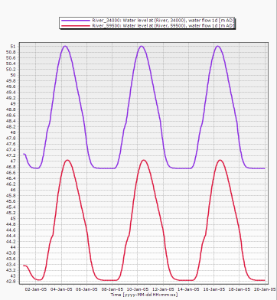
After running the model, right click anywhere on the network and select 'Query time series'. Then select, 'Water level'. A chart will pop-up with the requested time series.
If 'Query time series' is greyed out, first click 'select' and select the branch. Then click right again and select 'Query time series'. If you do not see 'select', right click closer to the branch.- Alternatively, double click on 'water level' in the output directory of the flow model in the Project Explorer. This will open the attribute table of the output coverage in the central map. With one or multiple records from this table selected, go to the 'map' tab in the Ribbon and click 'Query time series' from the Tools group. In this way, you should be able to create such graphs:
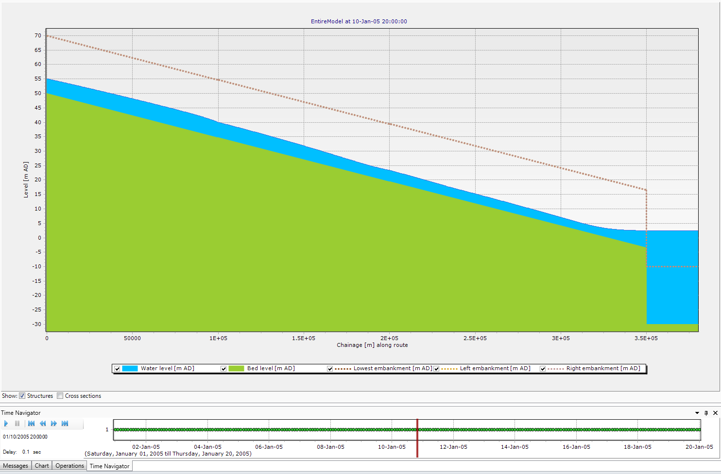
- Finally, let's revisit the sideview from the Add Cross-sections step 4-6. With the map open, open the sideview from the Ribbon. Below the sideview (in the same space as the Messages window), open the 'Time Navigator'. Inspect the progression of the flood wave by sliding the time navigator or pressing the 'play' icon:
This finishes this tutorial.