...
XBeach was originally developed for simulating the behavior of sandy coasts under extreme / energetic hydrodynamic conditions, specifically the processes of dune erosion (e.g. Van Thiel de Vries, 2009) and dune overwash (McCall et al., 2010). However, over the years several developments have lead to the very broad range of applications that XBeach is used for nowadays. XBeach is not only applied on sandy coasts anymore, but also on gravel coasts and coasts fronted by coral reef systems. And more recently, XBeach is being used to study erosion of (muddy) tidal flats. In addition to sandy, gravel, coral and muddy coasts, XBeach has been extended with a number of formulations to be able to simulate flow and waves on vegetated coasts (e.g. mangroves, sea grass, kelp etc.).

Example measured and computed wave height evolution for lab tests Kansy (1999),
with (measured: circles, model: solid line) and without (measured: squares, model: dashed line) vegetation.
Theory
General theory
This section describes the theory behind the current implementation in the XBeach model source code. However, at this moment code developments are ongoing, so this part is subject to change on a regular basis.
...
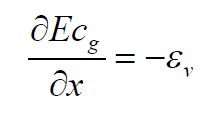 where E is the wave energy density, cg is the wave group velocity and εv is the time-averaged vegetation-induced rate of energy dissipation per unit horizontal area. A widely used method is to compute the time-averaged wave energy loss as the actual work carried out by the waves on the vegetation as function of the wave-induced drag force (e.g. Dalrymple et al., 1984):


where h is the water depth, αh is the vegetation height, F is the horizontal component of the force acting on the vegetation per unit volume, and u is the horizontal velocity. The overbar indicates averaging over time. When neglecting the plant swaying motion and inertial forces, the plant-induced force can be expressed with a Morison-type equation (Morison et al., 1950):

where ρ is the water density, CD is a drag coefficient, bv is the vegetation stem diameter, and N is the vegetation density. By applying linear wave theory to compute the horizontal component of the velocity, Dalrymple et al. (1984) found an expression for the time-averaged energy dissipation for regular waves propagation through a vegetation field on a uniform bed. This expression was extended by Mendez and Losada (2004) to include random waves, and waves propagating over a sloping bed, given by:


where k is the wave number, g is the gravitational acceleration, σ is the wave frequency, h is the water depth, CD is the (bulk) drag coefficient and Hrms is the root mean square wave height.
Damping of short (wind) waves
To take into account the damping effect of vegetation on the incident waves, the expression derived by Mendez and Losada (2004) was added to the short wave action balance:
 where A = Ew/σ, Ew is the wave energy, Dbreak is the wave dissipation due to breaking and Dveg is the wave energy dissipation due to the presence of vegetation, which can be computed using Eq. [4], and where the root mean square wave height is given by:

Following Suzuki et al (2011) the expression was slightly adjusted to take into account vertical layering of the vegetation:

where Dveg is the total short wave energy dissipation due to vegetation, nv is the number of vertical vegetation segments and Dveg,i is the short wave energy dissipation due to vegetation layer i:

By using this expression not only vertically uniform vegetation (e.g. sea grass) but also vegetation with a (strong) variation in characteristics over the vertical axis can be modeled (e.g. mangroves).
Damping of long (infragravity) waves and flow
...