Page History

...

At the moment of writing this page, during the 2nd technical meeting of the Technical Work Group of EMODnet in the Sea Aquarium of Genova in July 2017, the technical workgroup is discussing discussions about improvements on the services are the main topic. Until now the different EMODnet lots have carried out a great job to collect and harmonize all kind kinds of datasetsdata sets. Now it is the time to invest in harmonizing all portal portals so end users can find data a bit better.
At this technical meeting Deltares gave a presentation where a Use Case the use case presented got much attention. The Use Case was "I want to visualise the relation between the sea floor and the occurrence (with depth) of a specific animal (example is for Amphiura filiformis)". Some constraints were formulated, these are:

use the metadata delivered by the central portal (http://emodnet.eu --> product catalogue)
only by using OGC services
only by using free searches on species names

A stepwise step wise approach was followed to work out the use case is as follows. Steps followed:

go to the catalogue of EMODnet to find the data sets, these are:
1. bathymetry
2. biotic observations (without some specific knowledge it is hard to find datasetdata set(s) where abundance information of Amphiura filiformis can be found)
Go to the specific subportals sub portals via the links presented above and find out which services are available, these are:
1. for bathymetry the following services are made available
  
  WCS gives you the real data. The example will be worked out for this service. Find out more about WCS at the page WCS primer.
2. for biotic observations the challenge is to find abundance information on the VLIZ geoserver
  Geoserver can advertise WMS, WFS and WCS information, in case of species distribution in relation to depth the real observations are the way to go. Read more about WFS at the WFS primer page. Checking the complete geoserver and filtering on Eurobis it reveals the best dataset data set to be used is Aggregated points (stations) of EurOBIS occurences.
At this point insight is gained in the available sources and possible datasets data sets that can be used. Close investigation reveals however that the links offered for Bathymetry is are not really usable. Reverse engineering via the downloade download area of interest button on the EMODnet bathymetry portal reveals that the dataset data set with the real data is not advertised. This is shown via the get capabilities request of the WCS services provided.
Code Block
language xml
title WCS GetCapabilities
http://ows.emodnet-bathymetry.eu/wcs?service=WCS&request=GetCapabilities&version=1.0.0
this gives:

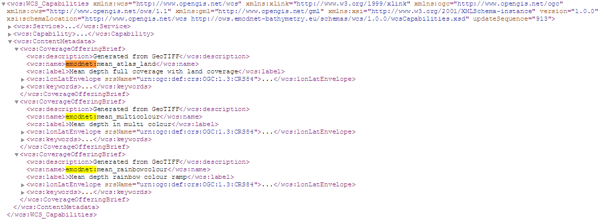
The developer tools gives information that a different layer is used, the coverage emodnet:mean is not mentioned in the getCapabilities but is used as layer to download.
Now a list of exact datasource data sources is know, these are:
1. for bathymetry (http://ows.emodnet-bathymetry.eu/wcs? coverage emodnet:mean)
2. for biota (http://geo.vliz.be/geoserver/Eurobis/ows? layername=Eurobis:eurobis_points)

On the primer pages present code snippets for python. These code snippets are adjusted to the particular example presented here.

Code Block

language	py
title	WCS code snippet

# import packages
import os
from owslib.wcs import WebCoverageService
from osgeo import gdal
 
# define the connection	
url = 'http://ows.emodnet-bathymetry.eu/wcs?'
wcs = WebCoverageService(url,version='1.0.0',timeout=320)
wcs.identification.type
wcs.identification.title
 
# define variables
clipfile = r'..\temp.tif'
requestbbox = (2.097,52.715,4.277,53.935)
layer = 'emodnet:mean_atlas_land'
 
# get the data
bathyml = 'emodnet:mean'
sed = wcs[layer] #this is necessary to get essential metadata from the layers advertised
sed.keywords
sed.grid.highlimits
sed.boundingboxes
cx, cy = map(int,sed.grid.highlimits)
bbox = sed.boundingboxes[0]['bbox']
lx,ly,hx,hy = map(float,bbox)
resx, resy = (hx-lx)/cx, (hy-ly)/cy
width = cx/1000
height = cy/1000

gc = wcs.getCoverage(identifier=bathyml,
		 bbox=requestbbox,
		 coverage=sed,
		 format='GeoTIFF',
		 crs=sed.boundingboxes[0]['nativeSrs'],
		 width=width,
		 height=height)

fn = clipfile
f = open(fn,'wb')
f.write(gc.read())
f.close()
filetiff = gdal.Open(clipfile)
theImage = filetiff.GetRasterBand(1).ReadAsArray()
os.unlink(clipfile)

for querying the WFS following code is used

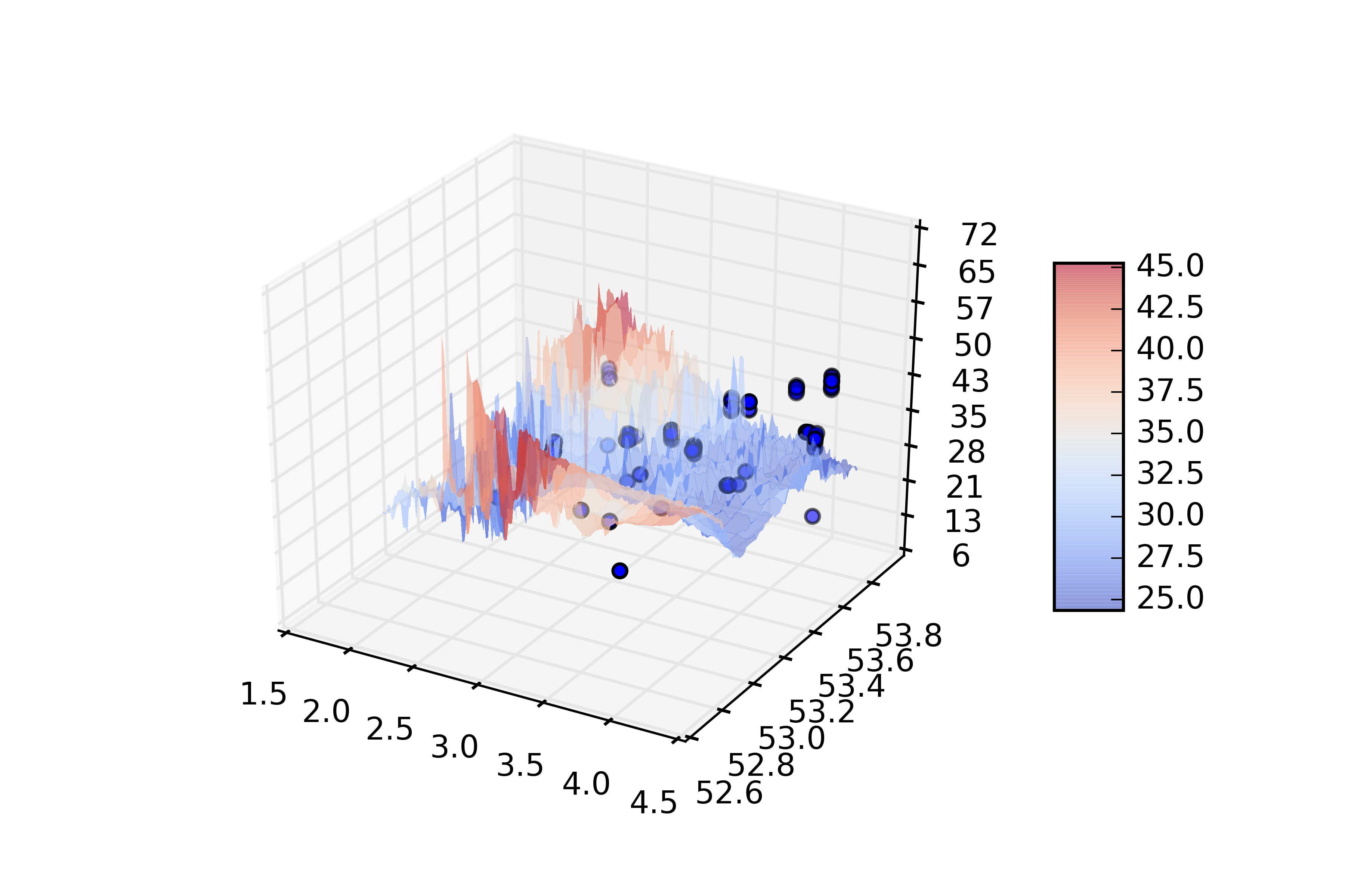
Code Block

language	py
title	WFS querying

# import the packages
import pandas
import sys
import os
from owslib.fes import *
from owslib.etree import etree
from owslib.wfs import WebFeatureService
 
# define the input variables
requestbbox = (2.097,52.715,4.277,53.935)
fn = r'..\afile'
wfs = 'http://geo.vliz.be/geoserver/Eurobis/ows?'  
layer = 'Eurobis:eurobis_points'
afilter = PropertyIsEqualTo(propertyname='Eurobis:ScientificName', literal='Amphiura filiformis')

# define the link to the service and carry out the request
wfs11 = WebFeatureService(url=wfs, version='1.1.0',timeout=320)
response = wfs11.getfeature(typename=layer, bbox=bbx,srsname='urn:x-ogc:def:crs:EPSG:4326',outputFormat='shape-zip')   
if os.path.isfile(fn):
    os.unlink(fn)
out = open(fn, 'wb')
out.write(response.read())
out.close()
    
# define pandas dataframe for the output
out = open(fn, 'wb')
out.write(response.read())
out.close()
df = pandas.read_csv(fn,header=0,sep=',')
os.unlink(fn)

Now the result (if there is data in the boundingbox, there is no testing involved, zou thus the result can be empty, this is not tested) is there, in 2 objects (Pandas DataFrame with observation information and a Numpy array with bathymetry). This can be plotted in a 3D Scatter plot using the Matplotlib. See next code.

Code Block

language	py
title	Plotting the data

img = theImage (see above)
bbox = requestbbox (see above)
def plotraster(img,df,resx,resy,bbox):
    from mpl_toolkits.mplot3d import Axes3D
    import matplotlib.pyplot as plt
    from matplotlib import cm
    from matplotlib.ticker import LinearLocator, FormatStrFormatter
    import numpy as np
    
    fig = plt.figure()
    ax = fig.gca(projection='3d')

    #plot the vectors
    xv = df['Longitude']
    yv = df['Latitude']
    zv = df['MaximumDepth']
    ax.scatter(xv,yv,zv,label=df['ObservedIndividualCount'])
    
    # Make data.
    X = np.linspace(bbox[0],bbox[2], img.shape[1])
    Y = np.linspace(bbox[1],bbox[3], img.shape[0])
    X, Y = np.meshgrid(X, Y)
    #R = np.sqrt(X**2 + Y**2)
    #Z = np.sin(R)
    Z = img
    # Plot the surface.
    surf = ax.plot_surface(X, Y, Z, cmap=cm.coolwarm,
                           linewidth=0, antialiased=False,alpha=0.5)
    
    # Customize the z axis.
    ax.set_zlim(Z.min().round(), Z.max().round())
    ax.zaxis.set_major_locator(LinearLocator(10))
    ax.zaxis.set_major_formatter(FormatStrFormatter('%.f'))
    
    # Add a color bar which maps values to colors.
    fig.colorbar(surf, shrink=0.5, aspect=5)
    plt.savefig(r'd:\temp\emodnet\test.png',dpi=600)
    
    plt.show()

The result is visualised in the following graph

...

Space shortcuts

Child pages

Versions Compared

Old Version 3

New Version 4

Key