
 This project has received funding from the European Union’s Seventh Framework Programme for research, technological development and demonstration under grant agreement no 607131.
Introduction
The MI-SAFE software and webviewer are developed under the EU funded FP7 project FAST (Foreshore Assessment using Space Technology). The MI-SAFE viewer depicts the estimated contribution of coastal vegetation to wave height attenuation for user-selected coastal locations anywhere in the world. The MI-SAFE viewer is thus based on global datasets made available via open spatial services and presented in the web-viewer. The data from these global datasets are used to query the results of a modelling exercise conducted with XBeach for a range of different types of vegetated foreshores and a range of exposure to waves and tides. The results can be used to assess the requirements for the design of coastal flood protection measures with and without vegetation fronting those measures; they give a first estimate of the potential risk reduction that coastal vegetation has to offer with respect to specific coastal flood events on any particular shore across the world.
For background information about the viewer, the project and all the partners involved, please visit our website - http://www.fast-space-project.eu/
MI-SAFE illustrative summary
In the figure below, Figure 1, a general overview of the principles of the FAST project are illustrated. The data sources and products produced by the MI-SAFE tool are illustrated in Figure 2.
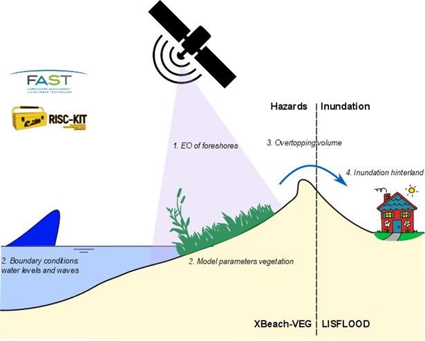
Figure 1. Illustration of the principles of the FAST project (linked to RISC-KIT project). EO = Earth Observation, XBeach-VEG = vegetation module of XBeach wave propagation model, LISFLOOD = hydrological model.
![]()
Figure 2. Figure showing the data sources and outputs of the MI-SAFE tool; data sources and calculations are explained below. Data sources indicated with an * are EO-based products from the FAST project. Hs = significant wave height; ERA-Interim = wave exposure dataset; XBeach = model for wave propagation, long waves and mean flow, sediment transport and morphological changes of the nearshore area, beaches, dunes and backbarrier during storms; GlobCover = global land use maps; CLC (Corine Land Cover) = European land use maps; GEBCO(General Bathymetric Chart of the Oceans) = bathymetry; TFA = ; SRTM(Shuttle Radar Topography Mission) = elevation
Links to methodological videos and public documents:
- Project flyers are available on the FAST project website: http://www.fast-space-project.eu/index.php/media-center/project-flyers
- Papers and popular articles published on the scientific advances made in the FAST project can be found here:
- A new Copernicus downstream service supporting nature-based flood defence (Deliverable D3.2) published in Sea Technology: https://www.researchgate.net/publication/280304012_Copernicus_Downstream_Service_Supports_Nature-Based_Flood_Defense_Use_of_Sentinel_Earth_Observation_Satellites_for_Coastal_Needs
- A new Copernicus downstream service supporting nature-based flood defence (Deliverable D3.2) published in Sea Technology: https://www.researchgate.net/publication/280304012_Copernicus_Downstream_Service_Supports_Nature-Based_Flood_Defense_Use_of_Sentinel_Earth_Observation_Satellites_for_Coastal_Needs
- Videos on FAST methods (i.e. field measurements, sensor deployment, etc., see Table 1), Nature, Events and Interviews can be found here: https://www.youtube.com/channel/UCy3pfgoHHmBU-vyd6yEkbzA
Table 1. Summary of methodological video clips available at the YouTube channel: FAST project.
Title / link | Description |
Installing a FAST field work site | Overview on how the FAST team install a fieldwork site. The video includes how the deployment of the measuring equipment is done for most of the methods used for field data collection. |
Sedimentation erosion table method | Instructions on how to measure how the sedimentation rate is changing with a sedimentation-erosion table (SET) |
Measuring Sediment Dynamics | Measuring sediment dynamics has been an important tool to study foreshores for years. The NIOZ developed and perfected special sensors for long term monitoring of these dynamics. This sensor uses 200 light sensors, and uses the difference between dark and light to determine the soil elevation. By measuring this continuously for months we gain valuable insights into both the small and large scale sediment dynamics. |
Side-on photography for vegetation analysis | Video demonstration of the use of side-on photography for vegetation analysis in salt marsh canopies. The method was originally developed for use in salt marshes by Möller (2000) and in parallel by Zehm et al. (2003) for grasslands, with further application for salt marshes reported by Möller (2006). Analysis of digital images obtained through the use of this method allows relative differences in the density, height, and structure of vegetation within a small area (in this case a rectangle of 0.2 x 0.6 m) to be compared across space or over time. Relationships between vegetation pixel density, as determined using this method, and biomass of salt marsh species have been suggested by Möller’s (2006) and Rupprecht et al.’s (2015) studies. |
Ground Based Spectrometry | A quick overview of how UCA makes ground-based spectrometry measurements to relate the reflectance properties of vegetation and sediments to satellites such as Sentinel-2. |
Processing Plant Biomass Samples | From sampling vegetation regularly on the study sites, the FAST team may detect seasonal changes on biomass, density and surface/weight ratios for dominant plant species on the intertidal area. This video shows how to process a biomass sample from intertidal areas to estimate these plant variables. |
FAST project on-line flood hazard tool: How to use MI-SAFE v0.1 | MI-SAFE is an on-line tool developed by the project. This interactive tool shows different layers of information based on satellite data and validated by field research. With the tool you can extract basic information such as the depth profile along a line or whether there are plants in an area or not. Eventually, this information is translated in the effect of the coastal areas and their plants on the height of waves inland. The first basic demo of this tool (MI-SAFE v0.1) has limited functionalities that are being expanded over the course of the project. The tool is available on-line at fast.openearth.eu |
MI-SAFE: Accessing products and services using the web viewer | In this video it is explained how to use the final version of the MI-SAFE viewer and access the underlying data layers. The tool is available on-line at http://fast.openearth.eu/index.htm |
MI-SAFE data
Elevation
Field data, local coverage
At each case study site, the topography of the surface has been recorded at a range of scales (from mm to 100s of meters). Alongside these measurements, observations of elevation change and accretion/erosion of surface sediments have been recorded at a number of specific locations on the marsh surface, some of which have been associated with the location of sampling quadrant used for sediment and vegetation measurements and field spectroscopy. Differential GPS (dGPS) surveys were conducted at each site towards the start and end of Year 1 and Year 2.

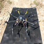
The FAST partners have also been testing out the use of unmanned autonomous vehicles (UAVs) for collecting very high resolution digital surface models of small areas. Whilst the technique requires careful calibration with insitu dGPS measurements, our first attempts have been very positive, suggesting that this may be a very useful technique to generate local scale elevation data.

Global SRTM coupled with GEBCO, Global coverage
Coastal and nearshore topography is an important factor determining the risk of flooding and thus features highly in the MI-SAFE application. The elevation of the surface over which the tides and waves travel determines how high the water level and the waves will be when they reach the most landward lying natural or artificial barrier. In addition, the type of surface and type of barrier determines how easily it is altered by tides and waves and how likely it is to suffer erosion. Hard rock coasts that rise up from the sea are less likely to suffer erosion than soft cliffs or sandy coasts. Topography and sediment stability therefore are very important factors. Several datasets are identified as useful for the characterisation of topography in FAST, these are:
- SRTM Topography (http://srtm.usgs.gov/)
- GEBCO Bathymetry (http://www.gebco.net/data_and_products/gridded_bathymetry_data/)
- ASTER (http://asterweb.jpl.nasa.gov/gdem.asp)
For the global version of the MI-SAFE viewer a derivative product called SRTM15_plus is used. It offers a continuous global coverage of bathymetry and topography. The SRTM15_plus dataset is created by the Scripps Institution of Oceanography (http://topex.ucsd.edu/index.html). This dataset is mainly used for viewing purposes since it is a continuous dataset at global level. For use in the MI-SAFE viewer a more detailed dataset is created using the SRTM3 v4 and GEBCO data (see Figure 3, vertical accuracy is about 15 m). The finest resolution of approximately 90 meter is combined where GEBCO is rescaled to 90 meter and interpolated to the SRTM tiles. To reduce computation time this is done for tiles along the OSM shoreline of the coast.
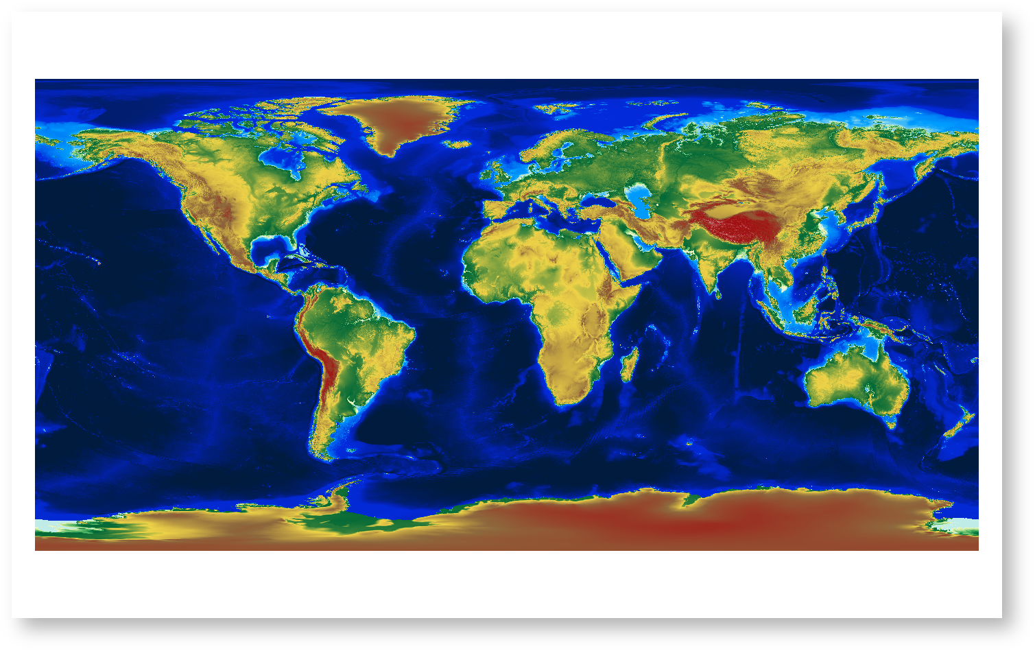
Figure 3. Combined SRTM + GEBCO elevation worldwide.
Inter-tidal elevation (satellite-derived), Global coverage
Precise elevation of the intertidal (foreshore) is crucial in the performance of the MI-SAFE viewer, because this is the area where the actual wave attenuation takes place.
Whilst in theory elevation and bathymetry data sources can be combined (see Elevation paragraph above) to create a continuous DTM that seamlessly covers intertidal regions, in practice a number of issues presently limit the usefulness of this approach:
- Intertidal regions are often missing from both land and seabed elevation data sets.
- Spatial and vertical resolutions may be below the minimum requirements of MI-SAFE (i.e. vertical accuracy of about 1 m).
- Most of the world is ‘data-poor’; meaning lower quality and reduced open-access to elevation data.
EU/ESA’s Copernicus, high resolution Sentinels (S1 and S2) and the NASA/USGS Landsat missions can help to fill this small, yet crucial gap. Extended temporal coverage means that a large number of images with different tidal elevations are available for most coastal regions. Identification of surface water (using indices and/or classification) from this large collection of images allows composite, time-ensemble averaged (TEA) images of the probability of inundation to be built up in tidal coastal zones. With calibration, these can be converted into inter-tidal elevation maps (Mason et al. 1995; Niedermeier, Hoja, and Lehner 2005; Murray et al. 2012). However, this technique is usually applied to relatively small regions and often includes in situ calibration via field measurements of intertidal elevation; hence the challenge for MI-SAFE was how to convert TEA inundation probability to elevation at a global scale without principally relying on field data?
To solve this challenge, as a first approximation, we assumed that:
- TEA water indices can be transformed to inundation probability [0,1] by normalising by the spatially-averaged, TEA water indices of regions identified as land and water, respectively.
- Once normalised, for a single pixel in an inter-tidal zone, the TEA inundation probability represents the long-term average of tidal height.
- If the inundation probability is derived from a collection of images that span a period of time similar to the tidal epoch, i.e., the time period over which tidal height statistics are derived (commonly 19 years), then pixels with a probability of 1 represent permanent water and have elevations less than or equal to the lowest astronomical tide (LAT), whereas land (p = 0) represents elevations more than or equal to the the highest astronomical tide (HAT). By deduction, p = 0.5 is then equivalent to mean sea level (MSL).
Development and production of inter-tidal elevation maps covering most of the global coast were carried out using the Google Earth Engine (GEE) computing platform; which facilitates rapid development and testing. The specific Open Access (OA) data sets used for product development are shown in Table 2.
Table 2. Earth observation and ancillary data sets used in this study. Abbreviations: United States Geological Service (USGS), European Space Agency (ESA), European Union (EU), Centre national d’études spatiales (CNES). Note pixel resolution is that used for the final product; other resolutions maybe available.
| Source | Provider | Name | Image collection ID | Date range | Resolution xy (m) |
| Google Earth Engine | USGS | USGS Landsat 5 TM TOA Reflectance (Orthorectified) | LANDSAT/LT5_L1T_TOA | Jan 1, 1984 - May 5, 2012 | 30 |
| Google Earth Engine | USGS | USGS Landsat 7 TOA Reflectance (Orthorectified) | LANDSAT/LE7_L1T_TOA | Jan 1, 1999 – ongoing | 30 |
| Google Earth Engine | USGS | USGS Landsat 8 TOA Reflectance (Orthorectified) | LANDSAT/LC8_L1T_TOA | Apr 11, 2013 – ongoing | 30 |
| Google Earth Engine | EU/ESA/Copernicus | Sentinel-2: MultiSpectral Instrument (MSI), Level-1C | COPERNICUS/S2 | Jun 23, 2015 – ongoing | 20 |
| Google Earth Engine | CNES-AVISO+ | Mean highest astronomical tide (HAT) 2005-2025, Global tide - FES2012 | users/edwardmorris1976/HAT | 2015 – 2025 | ~6000 |
| Google Earth Engine | CNES-AVISO+ | Mean lowest astronomical tide (LAT) 2005-2025, Global tide - FES2012 | users/edwardmorris1976/LAT | 2015 – 2025 | ~6000 |
Tidal statistics were derived from the GLOBAL TIDE - FES2012 model. Specifically, GeoTIFF’s with global coverage of mean LAT and HAT between 2005 and 2025 were derived from model simulations. These were added as “assets” to the Google Earth Engine platform for use in automated transformation of TEA water index images to inter-tidal elevation (Table 2).
For the purpose of validation and accuracy assessment we used insitu elevation datasets collected using dGPS at each of the FAST case study sites and high resolution digital elevation models (Table 3).
For the UK and NL sites, OA, quality Digital Terrain Models (DTM) generated by local authorities were available. For the Spanish FAST case study sites, available DTMs were deemed unsatisfactory (they had poor coverage in inter-tidal areas) hence a Unmanned Aerial Vehicle (UAV) flight from the Univ. Cadiz central services was commissioned and a high-resolution digital surface model was derived using structure-from-motion techniques for site ES_2.
Table 3. Insitu elevation data sets used in this study. Abbreviations: Foreshore Assessment using Space Technology (FAST), Univ. Cádiz (UCA), Univ. Cambridge (UCAM), Netherlands Institute for Sea Research (NIOZ), Actueel Hoogte Bestand Nederland (AHN), unmanned aerial vehicle (UAV), structure-from-motion (SfM). Note pixel resolution is that of the original data set; digital terrain models were bilinear re-sampled to 20 m.
| Source | Provider | Name | ID | Date range | Resolution xy (m) | Resolution z (m) |
| FAST project | UCA | In-situ dGPS elevation | FAST_ES_1_dgps_2014-2015 | 2014-2015 | 0.02 | 0.02 |
| FAST project | UCA | In-situ dGPS elevation | FAST_ES_2_dgps_2015-2016 | 2015-2016 | 0.02 | 0.02 |
| FAST project | UCA | UAV SfM digital surface model | FAST_ES_2_uav-sfm-1m-epsg25829_2015-2016 | 2015-2016 | 1.00 | 0.02 |
| FAST project | UCAM | In-situ dGPS elevation | FAST_UK_1_dGPS_Core_2014-2015 | 2014-2015 | 0.02 | 0.02 |
| FAST project | UCAM | In-situ dGPS elevation | FAST_UK_1_dGPS_Ancillary_2014-2016 | 2014-2015 | 0.02 | 0.02 |
| FAST project | UCAM | In-situ dGPS elevation | FAST_UK_2_dGPS_Core_2015-2016 | 2015-2016 | 0.02 | 0.02 |
| FAST project | UCAM | In-situ dGPS elevation | FAST_UK_2_dGPS_Ancillary_2015-2016 | 2015-2016 | 0.02 | 0.02 |
| FAST project | DATA.GOV.UK | Lidar composite digital terrain model | Donna Nook DTM | 2009-09-26 | 0.50 | ? |
| FAST project | DATA.GOV.UK | Lidar composite digital terrain model | Tillingham DTM | 2015-05-31 | 0.50 | ? |
| FAST project | NIOZ | In-situ dGPS elevation | FAST_NL_1_dGPS_Core_2014-2015 | 2014-2015 | 0.02 | 0.02 |
| FAST project | NIOZ | In-situ dGPS elevation | FAST_NL_2_dgps_core | 2015-2016 | 0.02 | 0.02 |
| FAST project | NIOZ | In-situ dGPS elevation | FAST_NL_2_dgps_Transect | 2015-2016 | 0.02 | 0.02 |
| FAST project | AHN | Lidar composite digital terrain model | Netherlands_Study_Site_Paulina:DTM | 2015-05-31 | 0.50 | 0.01 |
Work flow protocol and algorithms
The initial processing of optical images includes the transformation of at-sensor radiance to geometrically corrected (orthorectified) top-of-atmosphere reflectance, resulting in a level 1 product suitable for public use (Figure 4). During this process quality assessment (QA) and including per-pixel classification, such as clouds, may also be carried out; usually by the data providers i.e., USGS and Copernicus and provided as a QA band. Top-of rather than bottom-of (or surface) -atmosphere reflectance was used because more TOA scenes were available, and issues were observed with the standard atmospheric correction process in coastal regions.

Figure 4. Schematic diagram of the inter-tidal elevation product workflow. Ovals, boxes and diamonds represent data products, rules or properties and processes, respectively.
Further pre-processing included filtering for scenes that intersected an area of interest (AOI, see below), were collected within a specific time range (1997-01-01 to 2017-01-01), and excluding scenes with a metadata cloud cover value > 30 %. A relative cloud score was calculated using band combinations for each pixel of every image; pixels were set as cloud if they had a value > 90% of the time-averaged cloud score (per pixel) of the stack of images. When available, such as Landsat 8 OLI and Sentinel 2 MSI, pixels set as cloud, cirrus and shadows in the QA bands were also added to the mask, which was finally expanded by 3 pixels, before being applied to the image.
A number of approaches are available for mapping surface water using optical imagery; ranging from expert systems and evidential reasoning (Pekel et al. 2016) to thresholding based on normalised difference spectral indices (NDSI) (Boschetti et al. 2014; Donchyts et al. 2016). As a first approximation, in part because of the relatively low computational costs, we used a single NDSI, the modified normalised difference water index (MNDWI) (Xu 2006), which has been shown to be slightly more robust in vegetated systems (Boschetti et al. 2014); (SWIR1 - Green) / (SWIR1 + Green), where, SWIR1 and Green are the reflectance of the short-wave infra-red (~ 1600 nm) and green (~ 560 nm) bands, respectively. MNDWI values of land and water tend to be > and < 0, respectively, and were calculated for every non-masked pixel of every scene within the filtered image collection.
Considering each scene as a spatially-explicit measurement of tidal water inundation sampled from the tidal dynamics of that particular region, the temporal-ensemble of pixels at each point in space, is potentially a statistical representation of relative tidal heights. Thus, stacks of scenes were reduced to a single image by calculating the time-ensemble average of each pixel. Land and water ‘end points’ were automatically extracted from the histogram of mean MNDWI values and used to interpolate MNDWI values to inundation probability [0, 1] (with values outside the range of the end points masked). Of the remaining pixels values between 1 and 99% were retained, logit transformed and interpolated to the LAT (p = 0.99) and HAT (p = 0.01) values (m) relative to mean sea level extracted for the particular AOI from the global raster of tidal statistics.
Application to the global coastline
The global coastline was divided into ~ 25000 AOI of about 40x40 km2 using the OSM shoreline of the coast. AOI in polar regions were removed, as the technique is not suitable in areas with semi-permanent ice cover. Per AOI, all available scenes within the specified time range from the combined Landsat and Sentinel 2 collections were selected, filtered and processed to derive a single inter-tidal elevation (m, MSL) raster image. The median number of scenes per AOI was 315 (range: 2 to 2223). AOI with a low number of scenes were removed from consideration. As ancillary data, we also exported LAT/HAT, the histogram used for rescaling, the timestamps of the images used and a polygon-vector representing land (defined as elevation > MSL).
Product specifications
- Inter-tidal elevation: Each pixel represents a floating point value of time-averaged (1997 - 2017) surface elevation (m, relative to MSL) in the inter-tidal zone (between LAT and HAT).
- Land mask: This multi-polygon represents land which is inundated less than 50% of the time-period (1997 - 2017). In open coastal zones this is usually land with an elevation higher than MSL (although this is not always the case).
- Scenes were selected between 1997-01-01 and 2017-01-01; however the number of images, and their periodicity varied per AOI (median collection timestamp per AOI was 2010-02-25).
- The inter-tidal elevation raster product has a pixel (geometric) resolution of 20 m, however the input collections, Sentinel 2 and Landsat, have pixel resolutions of 20 and 30 m, respectively. Considering the variability in the number and periodicity of scenes, as well as per-pixel masking, every AOI potentially has a slightly different nominal resolution, however this must be between 20 and 30 m.
- The data products are produced as GeoTIFF raster files of intertidal elevation, GeoJSON multi-polygon geometry files of land-mask’s and CSV files containing ancillary data (per AOI).
- All geospatial products have a Web Mercator (EPSG:3857) datum/projection.
Quality, validity and accuracy assessment
The initial product generation resulted in a proportion (~ 15%) of AOIs that failed during the processing. For many of these there was an obvious explanation; they tended to be AOIs with no shoreline, either offshore or inland, or areas with no LAT/HAT predictions (such as the Caspian Sea). In general the product appeared to represent plausible inter-tidal topography in a number of tidal regions. Although, visual differences between adjacent AOIs were regularly observed, highlighting potential issues with using the self-contained AOI approach (Figure 5).
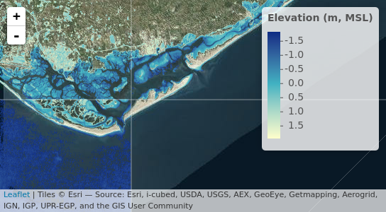
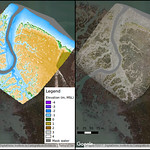
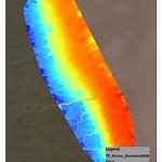
Figure 5. Map showing inter-tidal elevation of Ria Formosa, Portugal (AOI 164_030, 164_035 and 164_037, lat:36.98, long:-7.80).
Indeed, erroneous results were systematically observed in a range shorelines, mainly related to ‘false-positives’ in terms of identifying open water in the image collections. For example, volcanic substrates, which have MNDWI values similar to water, resulted in the false assignment of inter-tidal elevation. The same type of effect was also caused by snow cover and shadows from terrain. Errors of omission, e.g., known tidal flats not represented by the product, were also observed, for example in the Wadden Sea, NL. Here it is not directly clear why the technique failed, although the dynamic nature of the tidal flats might be an issue.
Quantitative validation and accuracy assessment was carried out by comparing predicted inter-tidal elevation values to in-situ data sources (Table 2) using the coefficient of determination (R2), root-mean squared error (RMSE) and mean absolute error (MAE). In-situ elevation data was supplied relative to an appropriate local vertical datum, roughly equivalent to ‘m above MSL’ at each site. For the ES, NL and UK sites, this was based on a local tidal station (Cadiz III), Normaal Amsterdams Peil (NAP) and Ordnance Datum Newlyn (ODN), respectively. Insitu dGPS measurements from both case study sites in each country (apart from micro-tidal RO) were combined with digital terrain model (DTM) data, bi-linear re-sampled to 20 m pixels, to allow an overall comparison of the accuracy of predictions (Figure 6).
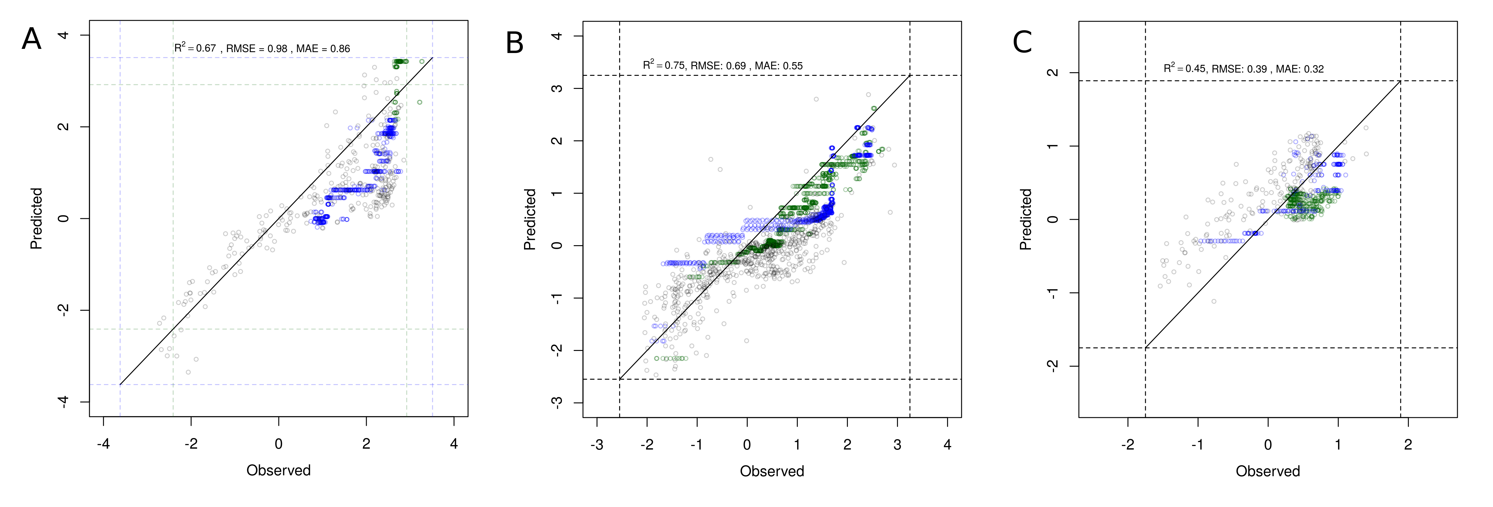
Figure 6. Scatterplot showing observed versus predicted inter-tidal elevation (m, MSL) at the case study sites. A) UK_1 and UK_2 on the east coast of the UK, B) NL_1 and NL_2 in the Westerschelde, SW Netherlands, C) ES_1 and ES_2 in Cádiz Bay, SW Spain. Green and blue points represent dGPS measurements (vertical accuracy of ± 0.02 m) from case study sites 1 and 2, respectively. Grey points are data derived from a high resolution DTMs (see Table 2), bilinear re-sampled to 20m pixels. Dashed lines represent LAT and HAT values for the region. Solid line is the 1:1 relationship. Statistical measures of ‘goodness-of-fit’ are also shown.
Coefficient’s of determination for a linear relationship between predicted and observed elevation ranged from 0.45 to 0.75, suggesting a reasonable fit. Examination of the scatter plots hinted at some non-linearity in the relationship towards the extremes of the inter-tidal ranges. RMSE and MAE values, estimates of the accuracy of predictions, ranged 0.32 to 0.92 m, suggesting predictions were generally within 1 m of the observed value. Particularly at the UK sites, which are separated by large distances, this maybe improved by further adjustments of the insitu data for ODN to MSL bias. To put in context the preliminary accuracy of the product, DTMs derived from Lidar often have a stated vertical accuracy of +- 0.2 m, whereas global DTMs tend to be in the 5-20 m range. Hence, this global 20 m pixel inter-tidal elevation product potential has accuracy between these 2 sources.
Waves
Field measurements, Local coverage
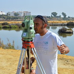
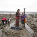
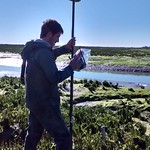
To acquire the results of the modelling exercise conducted with XBeach for a range of different types of vegetated foreshores and a range of exposure to waves and tides, the XBeach model was validated and calibrated against detailed water level data recorded using high frequency (4 Hz) dynamic water pressure measurements. This was done to resolve even small (2 Hz frequency) waves through the use of bed-mounted pressure sensors at a series of eight vegetated foreshores in Europe, ranging from reed beds in Romania (outer Danube Delta) to Sarcocornia salt marsh (Bay of Cadiz, Figure 7), and NW European estuarine and open coast salt marsh (The Netherlands and United Kingdom respectively). Data recording took place with a telemetered data logging system that captured waves and water levels during almost every inundation of the vegetated foreshores from early autumn to late spring over one year. The Romanian field sites Jurilovca (Razelm) and Histria (Sinoe) experienced continuous inundation, albeit with varying water levels, such that data acquisition at these sites varied from that at the United Kingdom, the Netherlands and Spanish sites with wave records triggered every 8 hours (three times per day). Water pressure records acquired in this way were processed into water depths, wave spectra, and summary wave statistics by the University of Cambridge, using tried and tested programming routines (Möller et al. 1996 and Möller and Spencer, 2002 ).
![]()
Figure 7. Transect in Cadiz (Spain) field site.
Era interim off-shore waves, translated to nearshore depth limited waves, Global/local coverage
Hydraulic boundary conditions in the form of off-shore wave data for return periods (Tr) of 1, 10 and 100 years are extracted from the ERA-interim dataset. Waves are generally lower in the tropics (e.g. less than 2 m between -30° to + 30°) than in temperate zones (where Hs>5m between 40°-70°). The picture below, Figure 8, gives a global view of wave heights for a return period of 1 year.

Figure 8. Global wave heights (Hs, m) with a return period of 1 year.
As the ERA-Interim wave data is based on offshore characteristics, waves are translated to onshore conditions by comparing the waves from ERA-Interim with a depth limited wave. If the depth limited wave height is smaller, this wave height is used for calculations whereas the period is maintained. The wave direction is not taken into account explicitly; the wave direction is assumed to be coast-normal, as it would be during a worst-case-scenario storm, for which an assessment of the protection function of the foreshore is likely to be most important. This approach seems to work well for exposed coastlines but likely leads to over-estimations of wave heights for more sheltered environments.
If more accurate hydraulic boundary conditions from the FAST case study sites were available, these were used as much as possible for the determination of the incoming wave height.
Water levels, Global/local coverage
Wave attenuation over foreshores is typically most relevant during storm conditions that create a surge (wind-induced water level set-up) in combination with high tidal levels. For the MI-SAFE viewer, a water level that has a probability of occurrence of 10%, i.e. once in 10 years, is considered to be the most relevant: this represents a storm that is both frequent enough to be relevant to users’ needs for planning coastal protection (a 1/100 or 1/1000 year condition may seem too extreme) and severe enough to be a serious threat to coastal regions. The representative water levels or hydraulic boundary conditions are derived from a global D-Flow Flexible Mesh model (Muis et al., 2016, Figure 9) that includes tides, storms and hurricanes. The output of this model is mapped to Dynamic and Interactive Vulnerability Assessment (DIVA) segments, so local anomalies can occur for coasts with irregular shapes (bays, estuaries). More extreme or locally tailored conditions are included in the Expert mode of the MI-SAFE viewer, which can take into account hydraulic boundary conditions that are specified by users -e.g. in local coastal management guidelines- or derived from dedicated modelling or field observations at the relevant location.

Figure 9. Global extreme water levels (tide + surge) for a return period of 100 years. From Muis et al. (2016).
Vegetation
Field data, local coverage
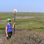
For each of the eight FAST case study sites (two each in Romania, Spain, the Netherlands, and the UK), vegetation species richness, percentage cover, and height was recorded seasonally in 1 x 1 m2 survey plots over a period of one year. In addition, a ‘photoframe’ was used to capture the density of the vegetation layer as seen from the side (and as experienced by water flowing over the surface). The vegetation photographed in this way also harvested (an area of 20 cm x 60 cm) to determine its biomass and, where appropriate (grass species), the number of stems per unit surface area. At the Romanian sites (Figure 10), tall reed was present and a sub-sample of stems was harvested from each survey location instead of using the photo frame area for harvesting.
In the MI-SAFE viewer this field data is used as input to the XBeach model. This was used to validate the performance of the XBeach model on the FAST case study sites and also to derive a set of representative vegetation characteristics per vegetation type (reed, marsh) for global application.

Figure 10. Vegetation measurements of the reflectance of reed beds in the Romanian field site.
Earth Observation products of vegetation, Global/local coverage
We provide the following vegetation products derived from Earth Observation:
- vegetation presence/absence (a global product)
- vegetation type (a product on European scale), and
- biophysical characteristics of the vegetation (examples for the FAST case study sites)
Vegetation presence/absence map, Global coverage
The amount and type of vegetation greatly influences how waves are attenuated as they cross the foreshore. To enable global foreshore assessments of wave attenuation by vegetation, a high resolution global map of vegetation presence and absence is paramount. Readily available maps such as GlobCover and Corine Land Cover (CLC) have resolutions that are too coarse (i.e. 200 to 300 m resolution) for the purposes of MI-SAFE, where a resolution of 10s of meters is required.
A global binary (presence/absence) vegetation map for coastal areas was created as input for the MI-SAFE tool and combined with GlobCover and Corine Land Cover to determine vegetation type (reed, marsh, mangrove). The presence of vegetation is determined using the Normalized Vegetation Index (NDVI) values which were calculated using Sentinel-2A and Landsat-8 products, using the Google Earth Engine (GEE).
Steps taken in order to derive a global vegetation map:
1) Coastline grids and sub-grids.
A global map is separated into grid cells and sub grid cells. Satellite images are collected only of the grid cells which contain a coastline. This helps prevent downloads and processing of redundant satellite images. Global coastline is derived from the OpenStreetMap website.
2) For each grid cell a cloud-free mask image is derived using QA60 band for Sentinel-2 and QA band for Landsat-8. Using this cloud free image collection NDVI value is calculated for each pixel in each image (esa.int). Pixels have a 10 m resolution for Sentinel-2 images and 30m resolution for Landsat-8 Images (Figure 11). For each pixel all available images are collected and stacked, i.e. image 1 till nth image. Per pixel, NDVI value is calculated for the entire stack for all available images. This gives an image collection of pixels containing NDVI-values for a specific x,y coordinate and for all different moments in time.

Figure 11. For each pixel all available images are collected and stacked, i.e. image 1 till nth image. Per pixel, NDVI value is calculated for the entire stack for all available images. This gives an image collection of pixels containing NDVI-values for a specific x,y coordinate and for all different moments in time.
3) Vegetation mask is built by defining a NDVI threshold for each x,y location. Based on the yearly NDVI average and NDVI amplitude, the threshold is chosen. This means that each location has a different NDVI value above which pixels are determined as vegetation, or non-vegetation. See Zhu et al, (2012) for a detailed explanation of this method.
The final product is in the format of a GTIFF (Figure 12).

Figure 12. Faro, Portugal. Vegetation mask is based on NDVI value larger than 0.3 for each pixel.
Vegetation type
Vegetation type is based on either GlobCover data (Global coverage, 2009) or Corine Land Cover (CLC, European coverage, 2000-2006) information that was reclassified to suit MI-SAFE needs (Figure 13). For non-temperate zones on a global level, a global distribution of mangroves map (Giri et al., 2011) indicates whether the vegetation encountered are mangroves or other vegetation. How the properties of the different vegetation types are characterized for the wave attenuation calculations in the MI-SAFE tool is described in 'Wave attenuation modeling: Characterising vegetation types'.

Figure 13. The four vegetation types on a map of the southwest of the Netherlands. The green areas in the upper right is the Biesbosch area with willows and reed beds. The yellow areas in the west are unvegetated intertidal flats in the Eastern- and Western Scheldt. At the fringes of these tidal environments, saltmarshes are visible in orange (e.g. 'Land van Saeftinghe') in the south and the FAST 'Zuidgors' fieldsite in the southwest, covered by blue lines.
Intertidal vegetation (salt marshes)
Intertidal vegetation is derived from the CLC class Salt marshes (421): areas submerged by high tides where vegetation dominates. The cover of such marshes can vary considerably between locations and throughout the year (Figure 14). For example, Spartina spp stands can well be 70 cm high during summer, whereas Salicornia spp. can be nearly absent in winter. The properties as observed by Möller et al (2014) were selected as representative, because they are for a mixed marsh typical for North-Western Europe and because they were measured with wave attenuation studies in mind rather than just observing biomass. Moreover, the drag coefficient of that particular vegetation cover has been derived from large-scale flume experiments under (near) real world wave conditions.
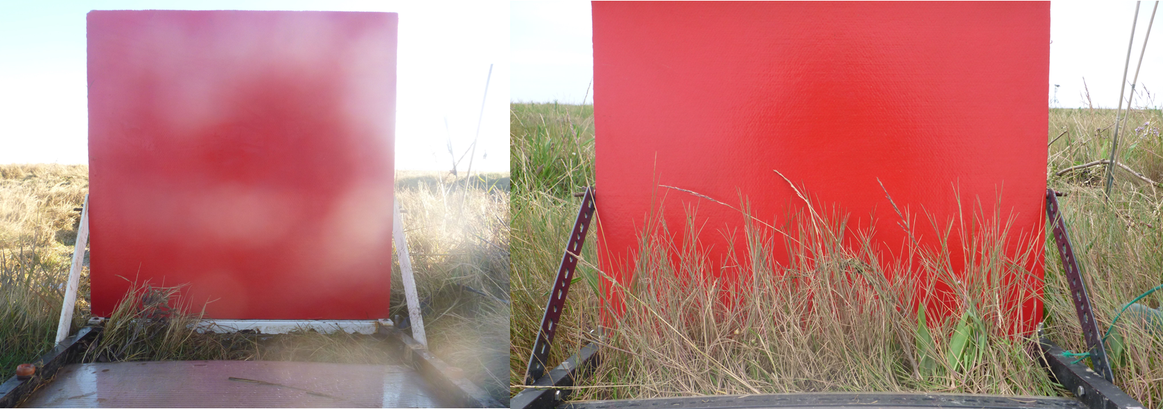
Figure 14. Salt marsh vegetation at the Tillingham (UK) marsh in winter (left; sparser and lower) and summer (right; higher and denser) 2015.
Inland marsh (reed beds)
Reed beds are of interest for inland locations such as lakes that are often fringed by reed beds, and for the Romanian study sites of FAST where large reeds grow in coastal lagoons. The CLC map does not account for reed beds as such, but are based on class 411 Inland marsh. As a result, the MI-SAFE viewer will apply reed bed properties to every inland marsh, also the ones predominantly made up of lower shrubs, and might overestimate the wave attenuation capacity of such marshes.
For the moment, the properties of the reed beds at the Romanian sites (Figure 15) have been used because these are readily available and because they represent the situation at the study site, which enables a comparison with local observations of wave attenuation. It should be noted that these are possibly taller reeds than usually found along lake banks.
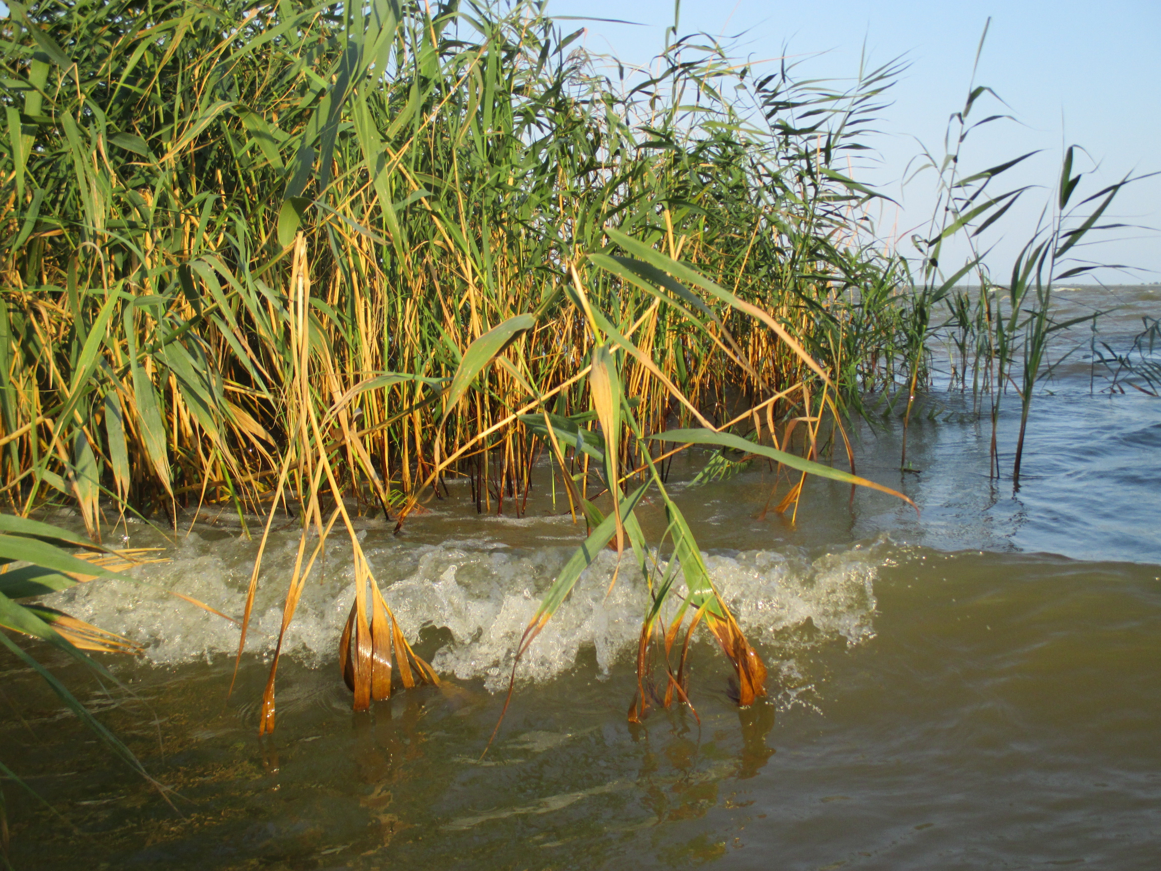
Figure 15. Wave breaking in Romanian reed vegetation.
Broadleaved forest (riparian willow forests and mangroves)
All areas classified by CLC as ‘broad leaved deciduous forests’ (class 311) are considered to be willow forests if they are located in Europe, where no mangroves occur. The CLC class also contains many forests far from any large water body, but these are not relevant as they will not be queried by users of the MI-Safe tool. Forests hardly occur directly adjacent to the coastline, and if they do they are usually coniferous so they will not lead to a false positive identification as willow forest. As a consequence, riparian forests are the most likely forests to be identified in this class. For areas outside Europe, the reclassified GlobCover data are further reclassified into willows in temperate regions and mangroves between -30° and +30° latitude. The world mangrove map of Giri et al. (2011) was not used to determine vegetation type because testing at several locations around the globe revealed that the location of mangroves on this map is not accurate enough for the purpose of the MI-SAFE viewer.
The composition, and consequently tree size, of riparian forests differs considerably among floodplains but willows are very common in European floodplains. The age and size of willows depends strongly on the management of floodplains: in natural rivers they are older and taller than along strictly managed rivers, where they can be cut regularly to prevent flooding as a result of the additional hydraulic resistance they cause. Such managed areas are more likely to be of interest, and the MI-SAFE viewer should not overestimate the wave attenuating effect. Therefore, the willow dimensions are chosen to be representative of relatively young, regularly trimmed trees. Data are available from sites in the Netherlands: commonly found regularly cut pollard willows (‘knotwilgen’) of several years old and young willows (less than 1 year old) of a field especially planted for wave attenuation in front of a levee near Fort Steurgat, Werkendam (Figure 16).
Like willows, the tree size and density in mangrove forests varies substantially among forests, depending on species composition and age of the forest. For the MI-SAFE viewer, the properties of the trees occurring at the seaward side (regular inundation, high salinity) of the mangrove forest are the most relevant because this is where most of the wave attenuation takes place. Moreover, further inland, the forest likely becomes more heterogeneous and mixed with terrestrial species. The two globally representative species for this zone are the red mangrove (Rhizophora spp.), which is characterized by prop roots (Figure 16d), and the black mangrove (Avicennia spp.), which is characterized by pneumatophores (Figure 16e). As deducing the type and size of mangrove trees from EO data is not (yet) possible, the MI-SAFE viewer relies on literature observations of dimensions of these two species, as summarized by Janssen (2016). To avoid overestimation of wave attenuation in young or very cyclic mangrove forests, the mangrove dimensions are chosen to be representative of young, pioneering mangroves up to 3 m tall.

Figure 16. Willows and mangroves used to characterize vegetation properties. a) and b) Pollard willows (~10 years old) that were measured in detail for an experiment on wave attenuation near Ridderkerk (NL). c) Young willows planted and measured by Deltares staff in front of a levee near Fort Steurgat (NL). Examples of d) red and e) black mangroves, which were characterized by Janssen (2016) based on a literature study.
Biophysical characteristics of the vegetation
The global methods to derive vegetation information give a broad overview of whether there is vegetation and the type of vegetation. However, with each of these types, the characteristics can vary spatially and temporally. To incorporate these variations into the MI-SAFE viewer, EO-based maps of the biophysical characteristics of the vegetation were created in different seasons and are visible in the data layers of the tool.
Biophysical characteristics: Normalised Difference Vegetation Index (NDVI) of the foreshore
One of the products of biophysical characteristics is NDVI, the Normalized Differential Vegetation Index (NDVI), of both the saltmarsh and the adjacent mudflat and waters. NDVI is based on surface reflectance in the red (RR) and near-infrared (RNIR) part of the electromagnetic spectrum, as follows: NDVI = (RNIR-RR) / (RNIR+RR). Hence, it has no units, and ranges from -1 to 1. As chlorophyll absorbs notably in the red, whereas the leaf structures of macrophytes scatter in the near-infrared, values typically increase with increasing cover, biomass or health of the vegetation. NDVI may also differ per vegetation type. Values of NDVI <0 typically indicate water. On the mudflat, higher values indicate higher biomass of microphytobenthos biomass, higher biomass, density and health or different types of macroalgae and seagrass. The product implemented in MI-SAFE is based on NDVI calculated from atmospherically corrected Sentinel-2 MSI images, for images of different seasons. Below are examples for such NDVI products at case study sites in the Netherlands (Paulina) and Romania (Jurilovca). In these products, land is masked. Spatial resolution of the NDVI product is 10 m.
Biophysical characteristics: Leaf Area Index (LAI) of the marsh vegetation
A core biophysical variable for the MI-SAFE viewer is Leaf Area Index of the marsh. Leaf Area Index refers to green leaf area per unit ground area. It is derived from Sentinel-2 MSI level 2B biophysical products. The algorithm for Leaf Area Index implemented in such level 2 products is based on a neural network approach, trained on a database of vegetation characteristics and associated Sentinel-2 top of canopy reflectances. The product as implemented in the MI-SAFE viewer refers to Leaf Area Index of the marsh only (where marsh is defined for NDVI>0.3). Areas outside the saltmarsh, either subtidal area or emerged tidal flat are set to 0, and land is masked. The maps can be produced for any vegetated foreshore, but in the MI-SAFE viewer, layers refer to the case study sites. See Figure 17 for examples for FAST case study sites in the Netherlands (Paulina) and Romania (Jurilovca) and Figure 18 for an example of seasonal variation of the marsh at Tillingham (UK).
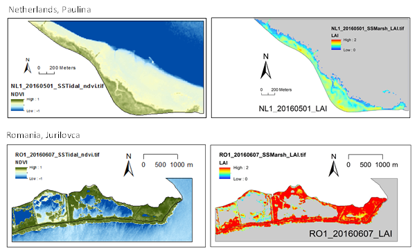
Figure 17. NDVI and LAI images for the FAST case study sites in the Netherlands (Paulina, upper two images) and in Romania (Jurilovka, lower two images).
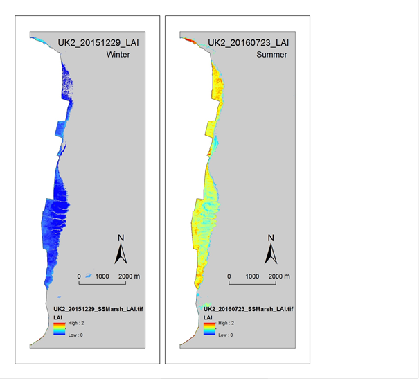
Figure 18. Seasonal variation in vegetation cover (LAI) at the Tillingham marshes. Left: December 2015, Right: July 2016. Darker colours represent higher LAI, i.e. more vegetation.
MI-SAFE tool services
The MI-SAFE viewer provides two main services on a global level:
1) Data layers from field and EO derived information, described in the sections above
2) Wave attenuation modeling outcomes translated into decrease in required crest height of a possible levee
MI-SAFE provides detailed information (10-20 m resolution) for FAST case study sites (Expert version). For other foreshore areas in the world the MI-SAFE viewer reverts to the global datasets mentioned above under 'MI-SAFE data' (Educational).
Wave attenuation modeling: General approach
In order to quantify wave attenuation by vegetation for a given salt marsh or mangrove coastline, the MI-SAFE viewer uses the numerical modeling software XBeach (van Rooijen et al., 2016). Xbeach is a depth-averaged, two-dimensional process-based model that solves the time dependent short wave action balance for the entire wave group, suitable for simulating wave attenuation over foreshores. XBeach has three wave energy dissipation processes relevant for MI-SAFE simulations: dissipation due to (depth-induced) wave breaking, dissipation due to bottom friction and dissipation due to vegetation. XBeach also has three simulation modes, from simple to advanced: stationary, surfbeat and non-hydrostatic. The stationary mode is fast but lacks wave groups (surfbeat) that are important for wave height variations near shore. The non-hydrostatic mode is physically the most complete but at substantial computational cost. The surfbeat mode does represent the effects of wave groups at reasonable computational cost and represents the effects of vegetation via the well known relations of Mendez & Losada (2004), and is therefore selected as the most useful mode for this application.
XBeach requires four parameters to represent the presence of vegetation:
1) Length or height h (m);
2) width or diameter d (m);
3) number of stems per horizontal area n (m-2);
4) drag coeffient CD (-).
The product of all parameters is the vegetation factor, which can be regarded as an 'effective biovolume' related to wave attenuation. The product of n, d and h is the leaf area index (LAI), which can be derived from EO. For deriving representative properties based on biophysical characteristics under 'Data', three principles were followed:
1) The vegetation factor should be relatively conservative, so as not to give an overly optimistic estimate of wave attenuation. Thus, plant dimensions are chosen with winter conditions and relatively small individuals in mind. The choice of the drag coefficient beforehand is troublesome, because this not only depends on the plant properties but also on the hydrodynamic conditions. Therefore, a relatively conservative estimate is made with large waves (that give large Reynolds/Keulegan-Carpenter numbers that are associated with low drag coefficient values) and the flexibility of the vegetation in mind. This can be refined once more reliable drag coefficient estimators are available, e.g. based on observations under (near-) design conditions in large-scale flume experiments.
2) The vegetation factor should be representative for all occurrences of a particular type, not just for a specific site.
3) The vegetation factor should be large enough and differ enough between vegetation types to meaningfully differentiate the effects of different vegetation covers from each other.
Wave attenuation modeling: Characterising vegetation types
In the table below (Table 4) it is shown how the different vegetation types are characterised in XBeach input parameters. Note that these basic assumptions are used if only global information is available in the Educational version of the viewer at present. In the Expert version, the local EO data are used to derive vegetation properties.
- For salt marshes, the values were defined based on the field observations at the FAST field sites, the properties of the temperate marsh tested by Möller et al. (2014) and the global inventory of Songy (2016). The drag coefficient of 0.19 is the lower limit found in the large flume tests by Möller et al. (2014); Songy (2016) matched field observations by Vuik et al. (2016) using a drag coefficient of 0.4. These values are well below the textbook value of ~1 for stationary flow through cylinders due to the flexibility of the vegetation.
- The mangrove parameters are based on the inventory of Janssen (2016), who synthesized observations of a.o. Cole et al. (1999), Narayan (2009), Mazda et al. (2006) and Horstman et al. (2012). Here, the representative drag coefficient could not be derived from experimental results since high quality observations on wave attenuation by mangroves under storm conditions do not exist. Instead, the theoretical value for a circular cylinder was used as mangrove trunks can be considered to be rigid.
- Reed beds are fully parameterized based on the observations at the Romanian field sites, the drag coefficient is chosen lower than 1 but higher than the 0.19 used for salt marshes to account for the greater rigidity of reeds.
- The properties of willows have been measured in two projects of Deltares (unpublished) along rivers in the Netherlands. For this vegetation type, the drag coefficient is chosen equal to that of mangroves, for the same reason of missing observations.
The calculated wave attenuation is very sensitive to the value of Cd (see example in Figure 19), so flume and/or field experiments that provide better estimations for this coefficient would greatly enhance the quality of simulations and thereby the applicability of nature based flood defenses.
Table 4. Vegetation input parameters to XBeach model. n = number of stems per m2 , d = diameter of the stems, h = height of the stems, CD = drag coefficient.
Type | n (m-2) | d (mm) | h (m) | CD (-) | nd (m-1) | vegetation factor (-) |
salt marsh | 1225 | 1.25 | 0.30 | 0.19 | 1.53 | 0.087 |
| mangroves | 30 | 35 | 3.0 | 1.0 | 1.05 | 3.2 |
reed beds | 77 | 10 | 2.6 | 0.60 | 0.77 | 1.2 |
willows | 15 | 8.4 | 3.4 | 1.0 | 0.13 | 0.43 |
Note that salt marsh vegetation has the lowest overall vegetation factor, but the highest nd, which means it is most effective at damping waves in shallow water. Willows have an opposite behaviour: in shallow water they are not as effective as in deeper waters. Mangroves with their root systems and canopy, and reeds with their vertically uniform structure are effective over a large range of water depths.
The example in Figure 19 below shows the importance of these processes on the FAST Tillingham (UK) field site, in combination with observations at this site as studied for FAST Deliverable 5.4 ('Prototype linkage of general rules for engineering requirements of dike design'). The thick black line indicates the bed level along a coast-normal transect, the thick green line the different vegetation covers observed. The thin black line represents the wave height change over the transect without bed friction or vegetation presence, i.e. purely depth-induced breaking. The thin blue, red and green lines represent wave height change in the presence of vegetation, for a range of vegetation drag coefficients. The dashed blue line represents wave height change in case of high bed friction due to very irregular small-scale bed topography (ridges and swales < 1m). Under these mild conditions (small waves, relatively low water depth), the attenuation by bed forms at the marsh edge dominates wave attenuation whereas under more extreme conditions (higher waves, deeper water) the attenuation by vegetation over the marsh plain will become more important.
For the Educational version, XBeach was used to generate a lookup table of attenuated wave heights for a range of possibly occurring combinations of nearshore waves and water levels, foreshore slopes and -widhts and vegetation types. The MI-SAFE viewer searches this table using the conditions at the selected site as input, resulting in a reduced wave height at the end of the vegetation where the levee is supposed to be. Subsequently, this reduced wave height is used to calculate a reduction in required crest height of the supposed standard levee, in comparison with a bare foreshore under the same forcing.
For the Expert version of the MI-SAFE viewer, a number (typically 6) of ~ 2 km long transects has been defined at each study site, running from the nearshore to the position of the levee estimated from EO images. At some sites (NL, UK) the foot of the levee can be clearly distinguished, on other FAST field sites (RO, ES) the relevant end of a transect is more difficult to define. For all transects, dedicated site-specific XBeach simulations have been performed using the local bed level, hydraulic boundary conditions and vegetation cover. Just like in the Educational version, this results in the attenuated wave height at the foot of the levee that is used to calculate the required crest height, but with much greater precision because the actual situation is simulated rather than a substantial simplification.

Figure 19. Outcome of XBeach model for various representations of salt marsh vegetation properties on the Tillingham field site, with bed level and wave heights.
Required crest height modeling
Wave attenuation over a foreshore is a very intuitive parameter, but solely assessing wave attenuation does not provide sufficient information about hazard -let alone risk- reduction because waves are not the only hazard. Most damage is actually caused by flooding resulting from high water levels. Therefore, many low-lying coastal areas are protected by a system of levees. The required crest height of such levees does not just depend on the water level but is also strongly related to wave height at the foot of the levee: Water flowing over the levee ('overtopping') resulting from wave run-up can erode the landward slope (Figure 20), thus threaten the geotechnical stability of the levee, as it reaches high velocities rushing down that slope. As vegetation on a foreshore typically gives lower waves at the levee foot, the required crest height height can be lower too, which means that the same level of flood risk reduction can be achieved at lower costs.
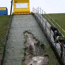
Figure 20. Failure of the inner slope of a levee as a result of a high overtopping discharge.
The calculation of required crest height (Rc) is based on empirical formulations described in Eurotop (Pullen et al., 2007). These relations form the basis of the official method for establishing required crest heights for levee designs and assessments in the Netherlands and other European countries. The Eurotop guidelines are the synthesis of a large number of experimental tests with varying levee geometries and hydraulic conditions that encompass most common levee designs. For a global analysis a different approach is required as in many places no coastal defence structures are present, or, if they are present, often properties of these structures are not known. Consequently, to be able to translate wave attenuation over a foreshore to a reduction of required crest height, several assumptions need to be made. First an allowed overtopping discharge needs to be chosen and second a standard schematisation of levee geometry for local hydraulic conditions needs to be assumed.
The allowed overtopping discharge (q) depends on the quality of the material of the levee, the resistance of the top layer and the incline of the inner slope. For example, good quality clay levees can withstand higher overtopping discharges than levees made of looser materials. Likewise, dense grass covers in good condition are more resistant than bare soils, but less resistant than asphalt cover layers. Steep slopes are less robust than gentle inclines because the water rushes down more rapidly and because of their inherently lower geotechnical stability. The allowed overtopping discharge is also related to duration of a design event (storm) as the deterioration of the inner slope is a time-dependent process. Here, we disregard the aspect of time is because of a lack of information on storm duration and to avoid a false sense of accuracy of the results. Experiments in large flumes and in the field have demonstrated the most resistant levees with good grass covers remain functional at overtopping discharges well above q=0.01 m3/s/m (Van der Meer et al., 2009). These are well-maintained levees in rich countries with vast engineering experience, so it seems unlikely that this is a representative value for global applications. A conservative choice of q=0.001 m3/s/m (Van der Meer et al., 2009) is more representative of simple earthen levees.
Given the lack of information on global levee properties, the calculations of required crest height in the MI-SAFE viewer are based on the (conservative) assumption that most levees have a basic configuration of a 1:3 outer slope without a berm and without substantial roughness or crest elements. For the design parameters at the toe of the levee, MI-SAFE calculates the wave height and water level (Figure 21) for the actual situations and a situation with an unvegetated foreshore. Subsequently, the MI-SAFE viewer uses these design parameters to compute the required crest height (relative to the still water level h) for both situations.
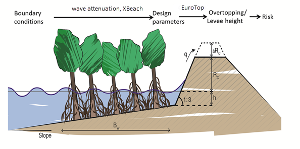
Figure 21. From boundary conditions to required crest height (with Bw = width of vegetation field, h = still water level, Rc = crest height, q = overtopping discharge) (adapted from thesis M. Janssen 2016).
The MI-SAFE viewer
The MI-SAFE viewer is built up of 3 main parts, these are:
- the canvas where the maps are shown
- the data part where a selection of layers can be toggled on or of
- the results.
Not yet mentioned is the back end of the dissemination platform which plays an important role in the data management of FAST. Figure 22 is a schematic representation of the MI-SAFE viewerl architecture. The base of the architecture is represented by a version control system based on subversion.
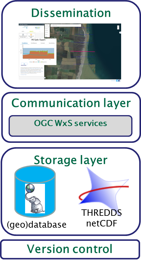
Figure 22. Schematic representation of MI-SAFE viewer architecture.
Subversion is used to store raw data, tools and imagery. Raw data and imagery can be placed in the storage layer whether or not after processing. The communication layer is middle-ware that converts data from the storage layer to web services, OGC WMS, OGC WCS, OGC WFS and OGC CAT ready to be disseminated via the viewer.
The MI-SAFE viewer consists of several components, already mentioned above. The pictures below, Figures 23 and give a good overview of the MI-SAFE interface and infrastructure.

Figure 23. Screen shot of the MI-SAFE viewer interface, 'Data' page. 1 = map canvas, 2 = layer selection, 3 = shortcuts to data from the FAST study sites, 4= search bar to navigate for a place of interest, 5 = zoom buttons, the + sign enables toggling between several background layers, 6 = quick access to metadata of the layer selected. Selected layers become green. Hovering over the link displays the abstract of the layer, 7 = legend of the last layer toggled on, it is possible to switch between legends on toggled layers by clicking on the legend icon on the right of the layer name, 8 = short cuts to FAST project Facebook and Twitter pages.
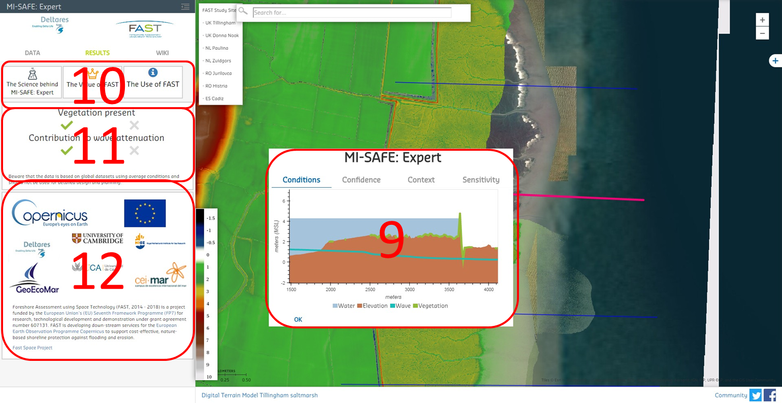
Figure 24. Screen shot of the MI-SAFE viewer interface, 'Results' page. 9 = MI-SAFE tool result showing several tabs: conditions --> physical condition on the study site or any particular place on the world (in the latter case resolution of the conditions visualised is less then for the study sites), confidence --> displays the quality of the information in terms of confidence, context --> gives context to the information displayed, sensitivity --> model result, 10 = Shortcuts to several sub pages where detailed information can be found, 11 = presentation screen indicating the effect of vegetation to wave attention (short version of the the outcomes of the tool results), 12 = project information; from any place on the screen the tool can be executed.
Actual processes and data retrieved via the MI-SAFE tool
The results part enables users to draw a profile of the coast. When a user queries a location in the MI-SAFE viewer combines data from four parameters to assess the effect of the foreshore on wave attenuation:
1) The local (sea)bed level;
2) The local water level, including tides and storm surge;
3) The local wave conditions;
4) The local vegetation type and cover.
The MI-SAFE viewer enables via WPS data retrieval over the profile via OGC services. To acquire these data for a queried location (point), the tool first determines a transect perpendicular to the nearest coastline. This transect runs 1000 m inland of the point where the bed level equals MSL and 1000 m seaward of this point; the area of interest where most wave attenuation occurs. This data is then used to query a pre calculated table of model results. The wave attenuation thus obtained is compared to the wave attenuation over a similar but bare transect. The result is shown indicating whether or not vegetation is existent in the intertidal and/or contributes to wave attenuation; the criterion for the latter is whether the situation with vegetation causes 20% lower waves than without vegetation.
MI-SAFE viewer results: Conditions, Confidence, Context and Sensitivity tabs
For the FAST case study sites assessed in the Expert version of MI-SAFE, the Conditions tab displays the bed level from local sources (e.g. DEM), the local water level (from local or regional hydraulic boundary conditions), the vegetation cover (from EO) and the change in wave height (from site-specific XBeach calculations) from offshore to the levee. In the Educational version, the same parameters are displayed but the bed level, waves, surge, vegetation type and cover come from global sources and the attenuated wave height comes from the closest match with schematized conditions in a look-up table with XBeach pre-calculated results.
The Confidence tab, similar in nature but different in contents for the Expert/Educational versions, indicates the origin of the various data sources (bathymetry, topography, wave height, surge or water level, vegetation presence and vegetation properties) by mouse-over and the confidence associated with these sources. The confidence is expressed in colours and linked to the detail, accuracy and particularity of the information:
- Green implies the highest confidence, typically for local DEMs based on LiDAR, local hydraulic boundary conditions and local LAI maps that account for spatially varying vegetation properties.
- Orange stands for e.g. TEA topography, hydraulic boundary conditions that apply to larger stretches (regional; multiple kilometers) of coastline and vegetation presence from EO combined with locally observed spatially uniform vegetation properties.
- Red means SRTM or GEBCO global data sources for bed level, a simple translation of ERA-Interim waves and GTSM surge levels to nearshore and vegetation properties based on standard vegetation types.
The Context tab describes and quantifies the conditions at the site (e.g. vegetation type encountered, length of vegetation field covered) and the hydraulic boundary conditions used (surge and wave height). This tab also compares the wave height of a vegetated foreshore with that on a bare foreshore and quantifies the required crest height for both situations, effectively giving an indication of the effect of vegetation on waves. For the Educational version, the required crest height is only calculated using the strictest overtopping criterion (q=0.1 l/m/s), for the Expert version also the required crest height using a less strict overtopping criterion is displayed to highlight the sensitivity of the results for this criterion.
The Sensitivity tab in the Expert version shows how different return periods (10, 100 and 1000 years) and different vegetation densities (bare, sparse, standard and dense) affect the required crest height of a (potential) levee. Note that this is the required crest height with respect to still water level (surge), not with respect to Mean Sea Level (MSL). The Educational version does not have this functionality.
Common MI-SAFE viewer issues
The algorithms in the MI-SAFE viewer have been developed and tested for many different situations around the globe. Still, there are situations that pose difficulties and lead to unrealistic results the viewer. These issues are usually due to data quality (e.g. elevation), complicated topography (e.g. bays, islands) or quick changes in time (e.g. rapid erosion, vegetation establishment). An illustration of common issues is listed in the table below.
| Issue type | Detailed issue | Location | Illustration |
|---|---|---|---|
| Temporal change; managed realignment | As a result of recent managed realignment, the foreshore is not recognized correctly and wave attenuation is not calculated over the present foreshore. Reasons: 1-The global coastline still follows the former (now outer) levee instead of the present levee. 2-The intertidal elevation map was made using images spanning multiple years; if the intervention occurred after this period, or caused ambiguous values, the area is not included in the map. If the area is not inundated regularly, the intertidal map cannot represent the elevation correctly, and the viewer reverts to using inaccurate SRTM topography. Solution: If this type of area is of interest, request application of the Advanced functionality that can incorporate any DEM, to the site. For an example of what results are possible, have a look at one of the FAST Study sites. | Freiston, UK |  |
| Temporal change or data quality | The viewer does not display the vegetation cover as observed by the eye of the user. Reasons: 1-The vegetation has established recently before the period used to construct the vegetation presence/absence map. 2-Part of the vegetation was covered by clouds and/or water during the period used for the construction of the vegetation presence/absence map. Solution: Request application of the Advanced functionality to the site, using recent and suitable Sentinel imagery for a site-specific vegetation cover. For an example of what results are possible, have a look at one of the FAST Study sites. | Freiston, UK |  |
| Complex topography; unclear coastline | Although the orientation of the transect in the viewer is correct, the resulting wave attenuation should be regarded with considerable caution: the algorithms in the viewer are made for a single water-land transition. Solution: Request application of the Advanced functionality to the site defining dedicated transects with output at meaningful locations and process-based calculations that can deal with complex topography. For an example of what results are possible, have a look at one of the FAST Study sites. | Blakeney, UK | 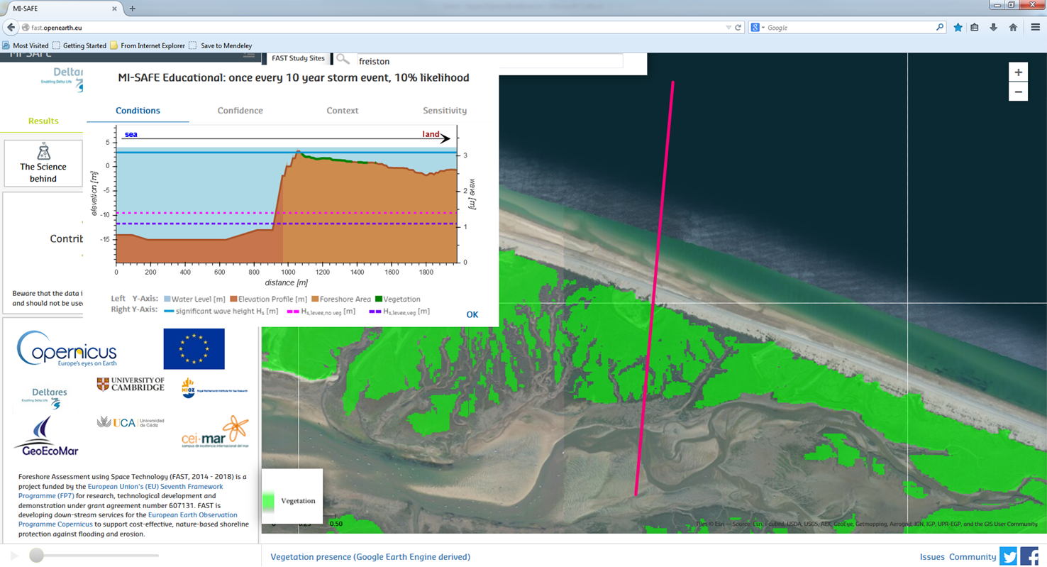 |
| Incorrect land elevation | The Sundarbans are a very low-lying area; land elevations around +10 MSL do typically not occur. The reason for the high observed elevation is that the SRTM topography used the reflection of the top of the mangrove canopy. Likewise, the intertidal elevation map cannot display this sort of area correctly, as waterlines underneath the canopy are not visible. | Sundarbans, Bangladesh | 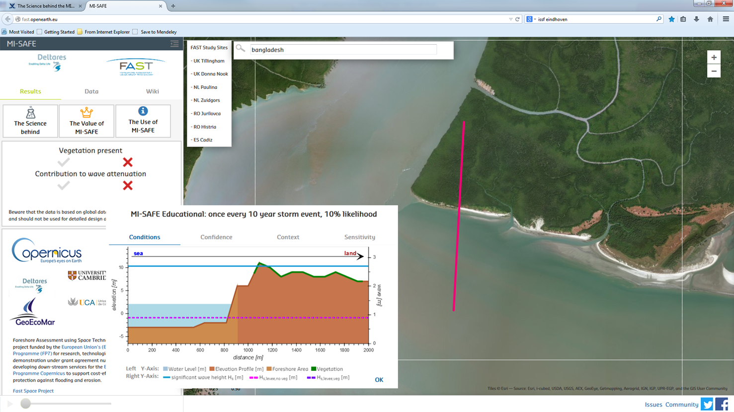 |
| Incorrect bathymetry | On some locations, the edges, i.e. the area near land, of the GEBCO bathymetry appear to be substantially deeper than the offshore areas. From other, not globally available bathymetry products such as EMODNET, we know that this is not true. Solution: On most locations the issue is cosmetic because the use of the intertidal elevation map provides a correct bathymetry where it matters; the calculations are meaningful but the transect looks strange. In the Advanced functionality, detailed bathymetric data can be used to ensure a correct transformation from offshore to nearshore waves. For an example of what results are possible, have a look at one of the FAST Study sites. | Bradwell-on-Sea, UK |  |
The case study sites
In the figure below, Figure 25, the location of the FAST case study sites are shown. In each red box, two locations are selected, leading to a total of eight case study sites in four countries.

Figure 25. Locations of FAST case study sites.
United Kingdom
Tillingham: This field site, Figure 26, is a macro-tidal (Mean spring tidal range of ca 4.8 m) open coast or outher estuarine salt marsh of the UK east coast (Southern North Sea) on the Dengie Peninsula in Essex. The estuaries of the Rivers Blackwater and Crouch lie to the north and south of the peninsula. The exposed marshes of this peninsula extend up to a maximum width of ca 700 m and are fronted by extensive intertidal mudflats, with an earthen embankment landward of them and low lying agricultural land behind this defence. Over the past 100 – 150 years the marshes have experienced several phases of advance and retreat. Marsh surfaces are composed of clayey silts and are approximately horizontal, with elevations of between 2.4 – 2.7 m ODN (Ordnance Datum Newlyn, which approximates to mean sea level). The Dengie Peninsula currently experiences rates of sea level rise of approximately 2 - 3 mm a-1 (Burningham and French 2011). The vegetation here is typical of UK east coast salt marsh with Aster tripolium, S. anglica, Suaeda maritima and Salicornia europaea present in the seaward areas. Higher up and further landwards, a canopy of P. maritima and A. portulacoides with E. athericus occurring on levees along creek margins is present. These species form mixed canopies but also exist in distinct mono-specific patches of several square metres in size, such that approximately uniform vegetation types can be found in close proximity to each other. Offshore wave heights have been estimated as averaging 1.09 m (on Long Sand Head, 42 km NE of Tillingham), with wave heights larger in winter (January), when mean monthly maxima reach 1.45 – 1.70 m (Herman 1999).
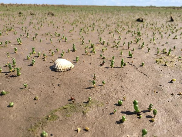
Figure 26. Tillingham field site in the United Kingdom.
Donna Nook: This site lies to the immediate south of the Humber Estuary on the East coast of the UK. It comprises a foreshore that consists of mixed clays, silts, and mud deposits and is occupied by a salt marsh in the upper regions. The marshes here extend out to a width of ca 750 m, with high exposure to winds from the north-east. The tidal range is 8.1 m at Immingham, providing water depths above the marsh surface at highest astronomical tide of between 0.9 and 1.4 m. Vegetation here consists of mixed north-western European salt marsh species (Atriplex, Puccinnellia, Elymus, Aster, Salicornia, and others). The marshes are flanked by extensive (> 1000 m wide) tidal flats to seaward and dunes and/or earth embankments on their landward margin. Evidence suggests a marsh progradation rate of 1-1.5 m per year over at least the past 5-10 years, through sediment derived from updrift (the Humber estuary and further north). Landward of the salt marsh for which data for FAST was obtained lies a recent managed realignment site (regulated tidal exchange through a breach in the most seaward embankment to create natural habitat to landward).
The Netherlands
The Westerschelde estuary is located in the southwest of the Netherlands. It has a macrotidal regime; discharge is relatively low compared to the tidal prism of the estuary. Wind-driven waves are particularly important at the mouth near Vlissingen, where fetch is longer. The Westerschelde has a salinity gradient from saline at the mouth near Vlissingen, to brackish at the Belgian border. The estuary is affected by human activities, such as dredging to facilitate navigation to the ports of Vlissingen, Terneuzen and Antwerp. The estuary is also part of a Natura 2000 area. It is characterised by a multiple channel system surrounding sandy and muddy tidal flats and shoals, as well as foreshores fringing the estuary, that are typically more muddy. These intertidal areas accommodate a large benthic community, providing food for birds and (flat)fish. At the higher parts of these tidal flats, saltmarshes can develop, consisting typically of Spartina spp in the more saline parts to Phragmites spp. in the brackish areas, mixed with other species. In EU FAST, we focused on two case study sites in the Westerschelde estuary, one sheltered, expanding saltmarsh (Paulina, see Figure 27), dominated by Spartina spp., and one wave-exposed, eroding (cliffed) saltmarsh (Zuidgors), consisting particularly of Elymus spp. and Atriplex spp. Both marshes are fronted by “bare” tidal flats and are backed by dykes.

Figure 27. Paulinaschoor field site in the Netherlands.
Spain
The Spanish FAST study sites are located within the inner system of the Bay of Cadiz. The Bay of Cádiz (Figure 28) is located in the west of the Gulf of Cádiz, SW Spain, between 36° 23’ to 36° 37’N and 6° 8’ to 6° 15’W. This area was declared a Natural Park in 1989 (and since then, it has been also declared as SPA, SAC and Ramsar site), having the particularity that the fringes of the Natural Park are highly urbanised.

Figure 28. Cadiz bay saltmarsh, field site in Spain.
The bay is divided into 2 basins, a shallower inner bay with a mean depth of 3 m mean low water (MLW), and a deeper outer bay with a mean depth of 12 m MLW (Rueda & Salas 2003). The area of the inner system is profusely occupied by salt marshes and the tidal flats in front of the salt marshes are inhabited by seagrasses. In this area, sediments are composed mainly of fine sand and mud, with a high organic carbon content (Carrasco et al. 2003, Rueda & Salas 2003). However, specifically in FAST study sites, the grain size is mainly composed of mud and silt. The entire system is strongly influenced by semidiurnal co-oscillating tides with mean amplitude of 1.5 m (Alvarez et al. 1997). For the inner system, the tidal exchange is relatively high, with average water turnover rates ranging from 50 to 75% per tidal cycle (Alvarez et al. 1997). The area of the bay is protected from the action of Atlantic swell by a barrier island (city of Cadiz), but it is clearly influenced by wind waves that generates waves up to 0.5 m (Hs, periods <5 s) on the fringes of the bay (tidal flats, with seagrasses).
Dominant saltmarsh vegetation on the intertidal area is mainly represented by Spartina maritima on the low saltmarsh and by Sarcocornia species (Sarcocornia perennis subsp. perennis; Sarcocornia fruticosa) and Halimione portulacoides (or Atriplex portulacoides) on the medium saltmarsh (García de Lomas et al. 2008). However, also other species like Suaeda vera and Limonium spp. can be found. Judging by historical data, the saltmarshes are rather stable and characterised by a complex patterned distribution (although detailed studies are not available).
Romania
Razelm-Sinoe Lagoon System is included in the Danube Delta, that is the final part of the Danube River (Figure 29). The average annual precipitation in the Razelm - Sinoe Lagoon is 350-400 mm/year, with a large evaporation which should lead to the raising of the ground water, saturated by chlorides and sulphates, and, consequently, to humid soils salinization.
The climate of the Lagoon System is continental, with hot dry summers and very cold winters. The water bodies from the lagoon system happen to be partly or entirely frozen during winter, with frizzing periods varying from days to week. Complete ice cover for long periods, however, is rare. The Lagoon System is located in one of the windiest areas in Romania.
During the past century, the system has been subject to major changes due to human interventions. These changes resulted into a complete change of the Lagoon specific ecosystems compared to its pristine state. Throughout a series of hydro-technical interventions, the Lagoon System has been transformed into a fresh water reservoir, to be used for agriculture and fresh water aquaculture, considered at that time much more viable economically.
The planned functioning regime of this hydrotechnic system was:
- between April 1 - June 1, water accumulates up to the level of +80cm;
- from June 1 to August 15, level maintained at +80 cm;
- between August 15 and September 15, the level - descended between +30 +50 cm to ease the fishing (fishing continues until October 30);
- between November 1 and March 30, the level of retention - maintained at +50cm (to “protect” the northern compartment from the brackish waters of Sinoe Lagoon).
All these hydrotechnical interventions have automatically led to drastic changes of the hydrological, hydrochemical and biological conditions of these lacustrine and lagoon ecosystems.

Figure 29. The Romanian field site.
Variations of the maximum and minimum water level regime
The hydrologic regime of the lagoon system is characterized by two specific elements, namely:
- a seasonal variation related to the seasonal variation of the Danube River regime (via the water regime of the Sf. Gheorghe branch)
- a variation related to the changes in the wind direction and intensity. The wind plays a major role in the water and sediments circulation between the parts of the lagoon system but also in the exchange at the remaining inlets (Edighiol and Periboina).
The highest frequency of strong winds is from N and NE – and under these conditions large water masses are circulated from the north of Razelm to the south which determines an increase of the levels at Jurilovca or Canal 5 and a level decrease at Sarichioi or Sarinasuf (Table 5).
Table 5. Quantitative descriptors and their respective indicators for presenting hydrological status of the Razelm - Sinoe lagoon.
| Descriptor and indicators | Quantity |
|---|---|
| Hydrological values | |
| Maximum Levels (prior to 1974 – year of closure of the Portita Inlet) | Goloviţa lake: +106 cm (March 11, 1970) |
| Maximum Levels (after 1974) | Razelm Lake: 153 cm (June 2, 1988) Golovita lake: 130 cm (January 9, 1981) |
| Absolute Minimum Levels (prior to 1974) | Babadag Lake: 16 cm (8-11.11.1969) Jurilovca: +9 cm (26.10.1959) |
| Absolute Minimum Levels (after 1974) | Sarichioi: +3 cm (December 26, 1986) Jurilovca: +8 cm (March 1, 1978) |
| Maximum Amplitude | 150 cm |
| Maximum Annual Amplitude | 120 cm (1988) |
References
Cole, T. G., Ewel, K. C., and Devoe, N. N. Structure of mangrove trees and forests in micronesia.Forest Ecology and Management, 117(1):95–109, 1999.
Horstman, E. M., Dohmen-Janssen, C. M., Narra, P. M. F., van den Berg, N. J. F., Siemerink, M., & Hulscher, S. J. M. H. (2014). Wave attenuation in mangroves: A quantitative approach to field observations. Coastal Engineering, 94, 47–62. doi:10.1016/j.coastaleng.2014.08.005
Janssen, M.P.J. (2016). Flood hazard reduction by mangroves. MSc. Thesis Delft University of Technology.
Mason, D. C., I. J. Davenport, G. J. Robinson, R. A. Flather, and B. S. McCartney. (1995). Construction of an Inter-Tidal Digital Elevation Model by the ‘Water-Line’Method. Geophysical Research Letters 22 (23): 3187–90. http://onlinelibrary.wiley.com/doi/10.1029/95GL03168/full.
Mazda, Y., Magi, M., Ikeda, Y., Kurokawa, T., & Asano, T. (2006). Wave reduction in a mangrove forest dominated by Sonneratia sp. Wetlands Ecology and Management, 14(4), 365–378. doi:10.1007/s11273-005-5388-0
Mendez, F. J., & Losada, I. J. (2004). An empirical model to estimate the propagation of random breaking and nonbreaking waves over vegetation fields. Coastal Engineering, 51(2), 103–118. doi:10.1016/j.coastaleng.2003.11.003
Moeller, I., Spencer, T., & French, J. R. (1996). Wind Wave Attenuation over Saltmarsh Surfaces : Preliminary Results from Norfolk , England.Journal of Coastal Research, 12(4), 1009–1016.
Möller, I., & Spencer, T. (2002). Wave dissipation over macro-tidal saltmarshes : Effects of marsh edge typology and vegetation change. Journal of Coastal Research, 521(SI36), 506–521.
Möller, I. (2006). Quantifying saltmarsh vegetation and its effect on wave height dissipation: Results from a UK East coast saltmarsh. Estuarine,Coastal and Shelf Science, 69(3–4), 337–351. http://doi.org/10.1016/j.ecss.2006.05.003
Möller, I., Mantilla-Contreras, J., Spencer, T., & Hayes, a. (2011). Micro-tidal coastal reed beds: Hydro-morphological insights and observations on wave transformation from the southern Baltic Sea. Estuarine, Coastal and Shelf Science, 92(3), 424–436. http://doi.org/10.1016/j.ecss.2011.01.016
Möller, I., Kudella, M., Rupprecht, F., Spencer, T., Paul, M., van Wesenbeeck, B. K., Wolter, G., Jense, K., Bouma, T.J., Miranda-Lange, M., & Schimmels, S. (2014). Wave attenuation over coastal salt marshes under storm surge conditions. Nature Geoscience, 7(10), 727–731. http://doi.org/10.1038/ngeo2251
Muis, S., Verlaan, M., Winsemius, H. C., Aerts, J. C. J. H., & Ward, P. J. (2016). A global reanalysis of storm surges and extreme sea levels. Nature Communications, 7, 11969. doi:10.1038/ncomms11969
Murray, Ni J., St. R. Phinn, R. S. Clemens, C. M. Roelfsema, and R. A. Fuller. 2012. Continental Scale Mapping of Tidal Flats Across East Asia Using the Landsat Archive. Remote Sensing 4 (11): 3417–26. doi:10.3390/rs4113417.
Narayan, S., Beck, M. W., Reguero, B. G., Losada, I. J., van Wesenbeeck, B., Pontee, N., … Burks-Copes, K. A. (2016). The Effectiveness, Costs and Coastal Protection Benefits of Natural and Nature-Based Defences. PloS One, 11(5), e0154735. doi:10.1371/journal.pone.0154735
Niedermeier, A., Hoja, D., and Lehner, S.. (2005). Topography and Morphodynamics in the German Bight Using SAR and Optical Remote Sensing Data. Ocean Dynamics 55 (2): 100–109. doi:10.1007/s10236-005-0114-2.
Pullen, T., Allsop, N. W. H., Bruce, T., Kortenhaus, A., Schüttrumpf, H., & Van der Meer, J. W. (2007). EurOtop, European Overtopping Manual - Wave overtopping of sea defences and related structures: Assessment manual.
Songy, G.M. (2016). Wave attenuation by global coastal salt marsh habitats. MSc. Thesis Delft University of Technology.
Van der Meer, J. W., Schrijver, R., Hardeman, B., Hoven, A. Van, Verheij, H., & Steendam, G. J. (2009). Guidance on erosion resistance of inner slopes of dikes from three years of testing with the Wave Overtopping Simulator. Proc. ICE 2009, (1994), 1–14. Retrieved from http://www.vandermeerconsulting.nl/downloads/2009_vandermeer_schrijver.pdf
Van Rooijen, A. A., McCall, R. T., van Thiel de Vries, J. S. M., van Dongeren, A. R., Reniers, A. J. H. M., & Roelvink, J. A. (2016). Modeling the effect of wave-vegetation interaction on wave setup. Journal of Geophysical Research: Oceans. doi:10.1002/2015JC011392
Vuik, V., Jonkman, S. N., Borsje, B. W., Suzuki, T., Kratzer, I., & Bouma, T. J. (2015). Nature-based flood protection: the efficiency of vegetated foreshores in reducing wave run-up. Coastal Engineering, 116, 42–56. doi:10.1016/j.coastaleng.2016.06.001