Introduction & summary
This tool calculates the sedimentation of an access channel over a certain period of time. The location and length of the access channel needs to be defined under 'Generic data' (as a structure with type: Access channel). Using the geometrical input of the access channel the initial profile over the full length is calculated. Based on the theory of Van Rijn (Basics of channel deposition/siltation, 2013) and the input parameters the sediment transport due to tidal flow and waves outside of the channel is calculated.
Subsequently, the trapping of bed load and suspended load is defined including resulting sedimentation within the channel. At the end of each calculation round the channel dimensions over the full length are updated and used as input for the following calculation round.

How to use the tool
- Open a new project
- Start in Generic Data by defining:
- Either a spatial varying bathymetry, or a coastline in combination with a cross-shore profile (slope)
- A wave climate
- Vertical and horizontal tidal characteristics
- Sediment characteristics.
- Only the wave climate is considered in the calculation (not the extreme waves)
- Nearshore wave climate is calculated based on linear wave theory in case an offshore wave climate is provided
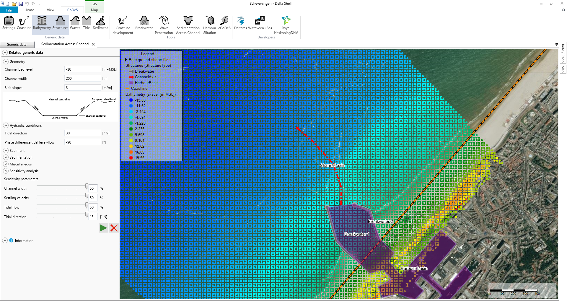
- Under “Structures”, draw a polyline element of type “Channel Axis”, if needed composed of several vertices

- Open the Sedimentation Access Channel tool
- Provide input according to the user input field description below
- Press the play button to start the Sedimentation Access Channel calculation
- After the calculation, a double arrow will be presented in the viewer indicating the tidal flow direction, which is an important user input variable (“Tidal direction”). The blue arrow indicates the flood flow direction and the white arrow the ebb flow direction.
Subsequently, subwindows are presented below the map which hold the following information:- Tidal conditions
This plot shows the Tidal water level [cm MSL] and the Tidal Current Velocity [cm/s] over 2 tidal periods. Time series of tidal water level and current velocity are based on the input data from Generic Data: tidal water level based on “MHW” and “MLW” and tidal current velocity based on “Maximum ebb flow” and “Maximum flood flow”. The input “Phase difference tidal level-flow” will define the time difference in phasing.
- Sedimentation Thickness
This plot shows the bed profile along the drawn Access Channel. It shows the Original Profile in red, the Dredged Profile in dark black and the Sedimentated profiles over the generated time steps. Average and maximum bottom level within the dredged section is also presented in the legend.
- Sedimentation Volume
This plot shows the total volume of sediment along the drawn Access Channel per linear meter. It shows the initial Dredged Volume in red and the total calculated sedimentation volume for each time step in grey. Total dredge/sedimentation volumes over the complete channel are also calculated and presented in the legend.
- Profile channel [Slider]
This plot shows a cross-section of the Access Channel at each of the calculation points. Using the slider below this plot it is possible to select a location. The plots include original bed level, initial dredged profile and sedimentated profiles for each calculation time step.
- Output properties
This panel shows a summary of the input parameters and calculated volumes: initial dredged volumes and sedimentation volumes for each time step. The last column presents the results from the sensitivity analysis for each of the included parameters. A comparison of the final thickness of the sedimentation layer and sedimentation volumes at the end of the simulation periods are presented here.
- Tidal conditions
Please be aware that the speed of the calculation scales:
- Linearly with the number of calculation rounds
- Linearly with number of calculation points
- When a sensitivity parameter is included (>0), 2 additional calculations will be executed including the lower and higher settings. Thus, including 1/2/3/4 sensitivity parameter will increase calculation time with a factor 3/5/7/9.
User input fields
A number of user input fields are provided which can be used to adjust the calculation according to the local situation. Default values are provided for each input field.
The following inputs are defined:
Geometry
| Default Value | Unit | Min. | Max. | Brief Description |
Channel bed level | -10 | m+MSL | 0 | -1000 | The initial bed level of the dredged channel. Check on deeper than local bed level |
Channel width | 200 | m | 0 | 1000 | Width of the bottom of the dredged channel at the start of the calculation |
Side slopes | 3 | m/m | 0 | 100 | The side slope of the channel indicated by 1 meter up, X meter to the side [1:X] |
Hydraulic conditions
| Default Value | Unit | Min. | Max. | Brief Description |
Tidal Direction | 30 | °N | -360 | 360 | Tidal flow direction during flood. Direction is measured compared to North (positive in clockwise direction) |
Phase difference tidal level-flow | -90 | ° | -360 | 360 | Phase difference in tidal level versus tidal flow. In case of 0° flow velocity is peaking together with the maximum water level. |
Sediment
| Default Value | Unit | Min. | Max. | Brief Description |
Suspended concentration Clay | 0.1 | kg/m3 |
|
| Clay concentration at upstream boundary (outside channel). |
Suspended concentration Silt | 0.005 | kg/m3 |
|
| Silt concentration at upstream boundary (outside channel). |
Settling velocity Sand | 0.02 | m/s | 0.005 | 0.05 | Settling velocity suspended sand (>50 microns). |
Settling velocity Silt | 0.001 | m/s | 0.0005 | 0.005 | Settling velocity suspended silt (10 to 50 microns). |
Settling velocity Clay | 0.0001 | m/s | 0.0001 | 0.0005 | Settling velocity suspended clay (< 10 microns). |
Sedimentation
| Default Value | Unit | Min. | Max. | Brief Description |
Method trapping efficiency | 1 |
| 1 | 2 | 1 – Method of Van Rijn 2 – Method of Eysink-Vermaas |
Coefficient Van Rijn | 0.26 |
| 0.1 | 0.4 | Coefficient Van Rijn |
Bulk method | 0 |
| 0 | 1 | 0 – Consolidation factor 1 – Constant value |
Bulk density Sand | 1.55 | ton/m3 |
|
| Sedimented Sand will occupy a volume according to this factor. |
Bulk density Silt | 1.12 | ton/m3 |
|
| Sedimented Silt will occupy a volume according to this factor. |
Bulk density Clay | 0.415 | ton/m3 |
|
| Sedimented Clay will occupy a volume according to this factor. |
Miscellaneous
| Default Value | Unit | Min. | Max. | Brief Description |
Total time period | 12 | month(s) |
|
| Simulation period in months. |
Calculation rounds incl. bed update | 2 | rounds | 1 | 10 | Number of calculation rounds equally divided over total time period. Each calculation round starts with updated bathymetry. |
Number of calculation points | 10 | points | 2 | 100 | Number of calculation points. The start and end of the channel and other vertices are always included. |
Sensitivity Analysis
| Default Value | Unit | Min. | Max. | Brief Description |
Sensitivity parameter: Channel width | 0 | % | 0 | 50 | Possible change or uncertainty in Channel width |
Sensitivity parameter: Settling velocity | 0 | % | 0 | 50 | Possible change or uncertainty in Settling velocity |
Sensitivity parameter: Tidal flow | 0 | % | 0 | 50 | Possible change or uncertainty in Tidal flow |
Sensitivity parameter: Tidal direction | 0 | ° | 0 | 15 | Possible change or uncertainty in Tidal direction |
Tool limitations
Linear wave theory is applied to translate offshore wave conditions into local nearshore conditions along the channel.
Influence of the channel on the propagation and dissipation of waves is not included in this analysis. Also the influence of bathymetric variety and structures on hydrodynamic flow and sediment transport are not included in this analysis. This will require more advanced numerical modelling.
Example cases
The following files (.dsproj) can be downloaded and loaded into CoDeS to serve as examples. They are not based on actual projects, but are intended as illustration.
Unzip the files to an convient folder (but make sure the file structure does not change), and open the .dsproj file from within CoDeS.