Monitoring of groundwater flow around a drinking water extraction well
Pieter Doornenbal (Deltares), Sjoerd Rijpkema (Vitens, now Waterbedrijf Groningen), Wiecher Bakx (Arcadis / Wetsus now Aveco de Bondt), Marios Karaoulis (Deltares), Edvard Ahlrichs (Deltares), Manos Pefkos (Deltares), Martijn Smeulers (Deltares), Mike van der Werf (Deltares now Metinco)
1. Motivation & Project goals
Around groundwater extraction sites, knowledge of the spatial and temporal behavior of groundwater is crucial. This is of particular interest to groundwater extraction companies and other groundwater users such as subsurface energy storage companies, farmers and water boards.
In the past years, research has been conducted to apply different measuring techniques to get insight in groundwater flow. Among these, active heating measurements with fiber optics as well as electrical resistivity tomography have shown a high potential towards measuring groundwater flow.
Vitens aims to obtain more insight around the flow of phreatic groundwater. In this specific setting, the water is relatively rich in iron, therefore the water company uses an underground iron removal system. There have been several research projects on the origin of the groundwater, however groundwater models investigating the groundwater flow are associated with high uncertainty estimates.
Groundwater flow is dependent on the porosity and composition of the subsurface, something which complicates obtaining accurate groundwater flow estimates and is associated with high error margins.
This project aims to provide greater insight into groundwater flow and groundwater flow direction around a drinking water extraction well using novel measuring techniques. The combination of these techniques has the potential to accurately determine groundwater flow and direction. These techniques could also be used to highlight the inaccuracies of groundwater models and complement them.
More specifically, the goal of the project is the development, implementation and demonstration of real-time groundwater flow monitoring using the relatively new active-heating Distributed Temperature Sensing (AH-DTS) and Electric Resistivity Tomography (ERT) technologies. Moreover, the possibilities of using highly advanced distributed acoustic sensing will also be explored. Successful implementation of these techniques will also increase knowledge regarding the issue of well clogging in groundwater extraction wells.
This project is aligned with the research project for the monitoring of groundwater flow. During the first phase of the project, lab experiments were performed, wherein an empirical relation was derived to relate temperature measurements to groundwater flow. The field experiments around a groundwater extraction well at ‘t Klooster (Vitens) aim to display the added value of applied measurements for the measurement of groundwater flow around an extraction well. In addition, the definition of subsurface heterogeneity derives from the measurements and can be incorporated into groundwater models.
2. Background
2.1 Active Heating Distributed Temperature Sensing (AH-DTS) Method
By using heat as a tracer, AH-DTS enables the direct measurement of groundwater flow velocities and direction in boreholes, in which fibre-optic cables are placed in direct contact with the aquifer. This method employs a fibre-optic cable to measure temperature in combination with a heating source, usually a separate heating element (as was done in this study), or injected water with an anomalous temperature. The relation between the transient temperature response and groundwater flow will depend on the thermal inertia of the passive cable (recording the ambient temperature) used to detect this response, the thermal properties of the lithology and the rate and direction of groundwater flow close to the cable.
In this study, the heating cables which were developed create a constant heat input for a fixed period of time. By measuring the temperature change occurring within that time frame, the maximum temperature difference with respect to the pre-heating period is obtained, which relates to groundwater flow velocity.
2.2 Electrical Resistivity Tomography (ERT) Method
The ERT technique is applied to get insight into the distribution of the resistance in the subsurface. Electrical currents are injected into the subsurface by electrodes, and the resulting potential is measured in two different electrodes. By measuring the drop in the potential, the ability of the electrical current to flow though the subsurface is determined, and so the electrical resistance can be defined. As the resistance can be related to the lithology and groundwater, this knowledge can be used to detect the subsurface composition and the quality of the water.
2.3 Distributed Acoustic Sensing (DAS) Method
Distributed Acoustic Sensing (DAS) instruments operate by sensing the acoustic field which interacts with the backscattered light generated along a continuous fibre optic cable. By analyzing the backscattered light and measuring the time between the laser pulse being launched and the signal being received, the iDAS can measure the acoustic signal at all points along the fibre.
The physical parameter measured by DAS systems is the rate of change of strain in the fibre (strain rate). This strain rate is averaged over a length of fibre equal to the gauge length, which is a fixed value, specific for each unit. It is important to note that the gauge length is different to the spatial resolution of the fibre optic cable, which is much finer, because the cable can be interrogated at intervals as fine as 0.25m.
By relating the amount of noise caused by the well to the recorded acoustics by the fibre optic cable we want to derive the feasibility of using this technology in groundwater flow.
3. What was done
3.1 Field Setup
3.1.a Development of an appropriate fiber optic measuring system
In order to complete the design of the AH-DTS system used in this study, laboratory measurements were necessary. Specific developments were made to ensure that the fiber optic system was optimally set up for the measurement purposes of the project.
A real-time active heating monitoring system was therefore developed (Figure 1), consisting of:
- Active heating unit
- DTS instrument
- Heating element/cables
- Fiber optic cable

Figure 1: The active heating monitoring system developed for the measurement purposes of this project
Prior to the main laboratory experiments, different types of fiber-optic cables including heating elements were tested and modeled. This included cable setups with a heating element within the mantle of the fiber-optic cable or separate from the fiber-optic cable. For the latter, variation was also introduced in the thickness of the fiber-optic cable protective elements (PVC and aramid protection).
The cable setup with a separate heating wire outside of the fiber-optic cable and relatively thin protective elements resulted in the highest ΔT groundwater flow velocity relation. Based on the results of this cable setup and modeling, an optimal active heating cable setup was constructed for the 2018 experiments.
Following the results of the laboratory experiments, the 2018 multi-mode duplex fiber-optic cable was developed (Figure 2) . This setup did not have a jacket and the two heating wires were glued directly to the fiber-optic cables. Heat in the heating wires was created by applying an electrical current to the wire and the resistance of the cable causing an even heating of the wire.

Figure 2: The cable setup developed for the laboratory experiments (Bakx et al., 2019) .
3.1.b Laboratory Measurements
AH-DTS has the potential to allow for the measurement of groundwater flow velocities in situ. We placed DTS fiber-optic cables combined with a heating wire in direct contact with aquifer sediments in a laboratory scale groundwater flow simulator (Figure 3). Using this setup, we empirically determined the relationship between 𝛥𝑇, the temperature difference by constant and uniform heating of the DTS cable and the background temperature of the groundwater system, and horizontal groundwater flow velocity.

Figure 3: Configuration employed in the 2018 laboratory experiments (Bakx et al., 2019)
Secondly, we simulated the observed temperature response of the system using a plan-view heat transfer flow model to calibrate for the thermal properties of the sediment and to optimize cable setup for sensitivity to variation in groundwater flow velocities. Additionally, we derived an analytical solution based on the heat flow equation that can be used to explicitly calculate flow velocity from measured 𝛥𝑇 for this specific AH-DTS cable setup.
We expect that this equation, after calibration for cable constitution, is valid for estimating groundwater flow velocity based on absolute temperature differences measured in field applications using this cable setup.
The results were published in 2019 in the Water journal.
3.1.c Development of an electrical resistivity tomography monitoring network
In order to develop the ERT monitoring network, surface measurements were first conducted at the ‘t Klooster site (Vitens). Using these results, we were able to configure the optimal position of the ERT electrodes relative to the wells (Figure 4).

Figure 4: ERT monitoring setup used in the field site.
4. Field Acquisition & Methodology
To develop the appropriate field acquisition and methodology, we used the fiber optic laboratory measurement results and the initial ERT surface measurement results. The composition of the field setups are shown in figures 5, 6 and 7.

Figure 5: Layout of the monitoring setup at ‘t Klooster showing the AH-DTS, ERT and iDAS cables. Green circle indicates the extraction well.

Figure 6: Profile showing the N-S configuration.

Figure 7: Profile showing the W-E configuration.
4.1 Installation of the fiber optic cables and ERT cables in the field pilot
Due to the very coarse material (stones of ~15cm diameter) present in the subsurface of the field site, the drilling strategy had to be changed. Drilling pipes of 160mm were chosen and drilling was performed using the rotating airlift method. During the installation phase, we followed a routine of describing the drilling cores, followed by geophysical well logs characterizing the subsurface surrounding the well. Following the conclusion of these measurements, the fiber optic and ERT cables were installed in the wells.
4.2 Monitoring of groundwater flow
This task was complicated due to several problems during the field installation phase, during which the fiber optic and ERT cable installation would require a greater amount of effort. Instead of measuring one location for a longer period (as was initially proposed for a one-year period), it was decided to measure in multiple locations for shorter periods. This led to a better understanding of the local geology and the heterogeneity in groundwater flow between different monitoring locations.
4.3 AH-DTS
The AH-DTS monitoring ran over a period of a week. Cables were installed in a total of 16 locations down to a depth of ~40 m below surface level. The positions of the heating elements on the fiber optic cables, as well as the lengths of each heating section, vary for each location. The time periods during which heat was applied were also differentiated to get insight in the amount of applied heat to the fibre optic cables.
4.4 iDAS
The DAS results presented in this report are derived from an experiment during which hot water was injected in a small research well while groundwater was being extracted from one of the main Vitens wells (Figure 8). Several rounds of experiments of injection in a small well and extraction from the main well were performed. The collected acoustic data were down-sampled from 50 kHz to 1 kHz and the root-mean-square of the signal was calculated for 1 second intervals.

Figure 8: iDAS experimental setup for measurements. The black line represents the surface level, while the blue line corresponds to the water table.
4.5 ERT
Four electrode cables were installed in boreholes around a centre well where water was extracted and injected. Electrical currents are inserted in the ground and the potential is measured using a pattern of current injection and potential electrodes from all cables. The data are inverted to a resistivity image and continuous models.
5. Results
5.1 AH-DTS
5.1.1 Laboratory Experiment Results
For the laboratory results, comparison of the model and measurement data was conducted for three experimental runs in order to validate the flow patterns (Figure 9). The blue line shows the temperature as measured in the experiments, while the red line is the modeled temperature for the best fit solution. The dotted green lines present the variations of Ks that were calculated. A best fit between observations and model data was obtained for the thermal conductivity of the sediment Ks= 5.0 W m−1 K−1, within ranges (2–8.4 W m−1 K−1) found in literature.
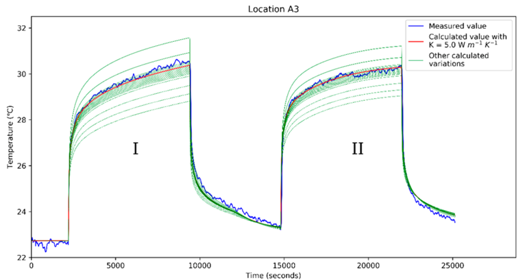
Figure 9: Comparison of model and laboratory measurement data (Bakx et al., 2019)
5.1.2 Field Measurement Results

Figure 10: Temperature results of AH-DTS measurements at several borehole locations close to the well in a N-S transect. The extraction well is situated between N11 and S14. Green Lines represent measurements taken when there was no groundwater extraction. Blue lines represent periods of groundwater extraction (presented at EAGE, 2020)
Figure 10 shows AH-DTS data at several locations near the extraction well. The temperature difference (ΔT) between the background groundwater temperature and temperature during heated is plotted. Two situations are shown in the figure: in green the ΔT without extraction and in blue the ΔT during extraction of groundwater from the central well. There is an increase of flow of groundwater to the well upon extraction, resulting in more cooling of the fibre optic cables. This is observed as a decrease in ΔT in figure 10. The well screen of this particular extraction well is situated between 17.8 – 32 meters below surface level.
As expected, the largest difference in ΔT can be observed over this interval. The top level, until a depth of ~ 9 to 14 m of cables S14 and S16 show identical ΔT results, because there is no well screen at these depths. Cable N11 shows a level at 25 m below surface level with a high ΔT that is identical in the cases with and without extraction. This is an indication of a local area of no flow.
Possibly this is a result of the local presence of clay or clogging. The cause needs to be investigated. The end of the groundwater flow zone at a depth of ~34 m can be observed in the two cables further away (N1 and S16) from the extraction well and slightly deeper in cable S14.
5.2 iDAS
Before the injection of the hot water, no signal was observed along the entire cable. At the onset of the injection and throughout its duration, there are vibrations recorded along the coiled interval of the fibre optic cable (yellow dashed section in Figure 8). These vibrations can be caused by either the petrol-powered generator at the surface to pump the hot water, or by the water itself flowing down the small borehole adjacent to the main borehole. There is a marked signal at time 165 s (at 135 s after the start of the injection), which propagates downwards (Figure 11). This is probably related to a thermal effect.

Figure 12: A zoomed-in section of the DAS data showing the area close to the bottom of the well (denoted by the black line) (presented at EAGE, 2020)
Figure 12 shows a zoomed in section of the straight fiber optic iDAS cable until the bottom of the well (denoted by the black line), and back up again. There is no signal recorded by the linear interval of the cable between distance markers 900 and 940 m. In order to better understand the acoustic signal, we need to process and interpret the DAS data of the other infiltration and extraction experiments. In conclusion, using a coiled fiber optic cable instead of a straight line is a potential alternative to increase vertical resolution and sensitivity.
5.3 ERT
ERT was found to be capable of imaging small changes in temperature, and patterns linked to the fluid flow. In Figure 13, the well screen is situated between 15 and 34 m below the surface, in the gravel part of the formation, and temperature variations derived from electrical resistivity from a water infiltration experiment are shown. When water is being infiltrated, temperature changes are visible in the depth range where the well screen is present. Because of the finer material above and below the gravel layer, we expect that the water will not go there and that is what we observe. It stays within the gravel layer.
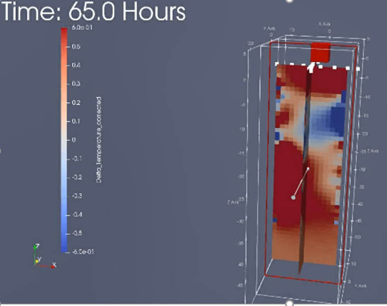
Figure 13: Temperature variations derived from electrical resistivity measurements
6. Discussion
6.1 AH-DTS
Figure 14 displays the measured ΔT groundwater flow velocity and the modeled groundwater flow velocity using measured ΔT as input shown for the 2018 experiments for optimized C and m constants, which are specific for the cable setup used in this experiment.
The equation in Figure 14 determines groundwater flow velocity using ΔT as input. The experimental data were inputted to determine the constants C and m, which vary for different setups. Using the estimated constants C and m, the equation was applied to estimate the groundwater flow velocity based on the measured ΔT.
The result is plotted together with the experimental results (mean values per groundwater flow velocity) for the 2018 data. The modeled groundwater flow velocity using the analytical solution results in a good fit to the measurement data for low ΔT (<7 ◦C) and higher flow velocities. For higher ΔT, the flow velocity is overestimated by the equation compared to the measurements.

Figure 14: Analytical solution derived for flow; m is a constant for cable setup.
6.2 iDAS
By analyzing the frequency content of the iDAS signal during hot water injection, it becomes clear that there is significant background noise contamination for frequencies below 220Hz (Figure 15). For this reason, in order to better investigate hot water injection, one should focus on frequencies higher than 220Hz.

Figure 15: iDAS signal frequency content.
6.3 ERT
The ERT monitoring experiment was performed during normal operation of extraction of groundwater and infiltration of oxygen-rich water in the purification step, during several weeks (14 September – 1 October 2018). The temperature difference between the ambient groundwater and the infiltration water was small, in the order of 1°C. This small temperature difference, however, caused detectable changes in the resistivity distribution in the aquifer (Karaoulis et al., 2019). During one of the infiltration phases (28 September 2018), the movement of the groundwater could be clearly followed via the changing resistivity patterns. A next step is to link the ERT and the AH-DTS data which were simultaneously measured.
7. Conclusion & Future Outlook
The examples shown here indicate that groundwater flow can be successfully detected using different fibre optic techniques and ERT. The AH-DTS data show that there is a difference in ΔT between situations of flow and no flow of groundwater. In addition, the zone of influence of groundwater flow, roughly coinciding with the well screen depth can be clearly distinguished in the data. The ΔT data will be converted into flow velocities. The DAS data show that there is an acoustic response during one of the infiltration experiments. The results from different techniques will be combined in the near future and then used to optimise the extraction and infiltration pattern of the well field. This is analysis is part of the follow project TKI GROFLOMO listed below
Follow up projects
The results of this TKI project are used to contribute to the following projects:
- TKI GROFLOMO
- Monitoring Piping experiments
- Monitoring fresh / saline interface Dunea
- Monitoring heat distribution Optigbes
Peer reviewed articles
This project contributed to the following peer reviewed articles
- Bakx et al. - 2019 - Determining the Relation between Groundwater Flow Velocities and Measured Temperature Differences Using Active Heat (Water 2019, 11, 1619)
- Bakx et al. (submitted 2021), Review: Measuring groundwater flow velocities near drinking water extraction wells in unconsolidated sediments
- Bakx et al. (under construction), Understanding groundwater flow velocity towards a drinking water extraction well by combining ERT and AH-DTS measurements
Presentations on conferences
This project contributed to the following presentation presented at conferences
- Bakx, Msc 2017, October 10th Wetsus Conference (Relating active distributed temperature sensing measurements to groundwater flow velocities in an experimental setup)
- Pieter Doornenbal, Pauline Kruiver, Edwin Obando-Hernández, Manos Pefkos, Marios Karaoulis, Wiecher Bakx, Francesco Ciocca, Athena Chalari, Michael Mondanos. 9-11 march 2020, First EAGE workshop on fibre optic sensing. (Fibre optic monitoring of groundwater flow around a drinking water extraction well)
- Marios Karaoulis, Wiecher Bakx, Pieter Doornenbal, Pauline Kruiver, Sjoerd Rijpkema Near Surface Eage 2019. Visualizing Groundwater flow using Time-Lapse Electrical Resistivity Tomography)
Acknowledgement
The results of the project were partly achieved within the collaboration in the Wetsus researchtheme "Grondwatertechnologie"