Invitation:
Prior to the 2015 NCK days icebreaker, OpenEarth.nl organizes a hands-on sprint session to explain how to access and visualize some great open access core-description and grain size datasets of the Dutch coast:
...
Flyer: NCK days 2015 sprintsession north sea grain sizes.pdf
| View File | ||||
|---|---|---|---|---|
|
Course information:
Access information for the data can be found at Dataset documentation.
You can download netCDF files (to prevent wifi overload) with BITSadmin. An example is for the TNO gain size maps is:
| Code Block |
|---|
set from=http://opendap.deltares.nl/thredds/fileServer/opendap/tno/ncp/
set into=d:\opendap\tno\

bitsadmin /transfer Job001 /download /priority normal %from%slib_juli2007.nc %into%slib_juli2007.nc
bitsadmin /transfer Job001 /download /priority normal %from%grind_fbr2007.nc %into%grind_fbr2007.nc
bitsadmin /transfer Job001 /download /priority normal %from%dz10_juli2007.nc %into%dz10_juli2007.nc
bitsadmin /transfer Job001 /download /priority normal %from%dz50_juli2007.nc %into%dz50_juli2007.nc
bitsadmin /transfer Job001 /download /priority normal %from%dz90_juli2007.nc %into%dz90_juli2007.nc |
You can access subsets these files with the Matlab netCDF package called ncread and with the python package netcdf4-python, see our Matlab example and
python example.
TNO grain size maps
A Matlab simple example how to make a publication quality figure is given here
| Code Block |
|---|
%% laod openearthtools for handy tools such as nc2struct, pcolorcorcen, colorbarwithvtext, tickmap, axislat, findfont
oetsettings
%% load data (local cache), D contains data, M contains all metadata
[D,M] = nc2struct('slib_juli2007.nc')

%% load data (via opendap)
L = nc2struct('http://opendap.deltares.nl/thredds/dodsC/opendap/deltares/landboundaries/northsea.nc')

%% plot
pcolorcorcen(D.longitude,D.latitude,D.mud)
colorbarwithvtext([M.mud.long_name,'[',M.mud.units,']']) % add text inside colorbar to maximize use of paper space. automatically use metdata from netCDF file
tickmap('ll') % add lat/lon as last tickmarks, no need for space, that dilute efficient use of paper space (google: Edward Tufte)
grid on
axislat % fix aspect ratio
plot(L.lon,L.lat,'k')
set(findfont,'fontsize',8)
title({M.nc_global.institution,'NCP map mud [version jul 2007]'}) % automatically use metdata from netCDF file as title
print2screensize('slib_juli2007')
|
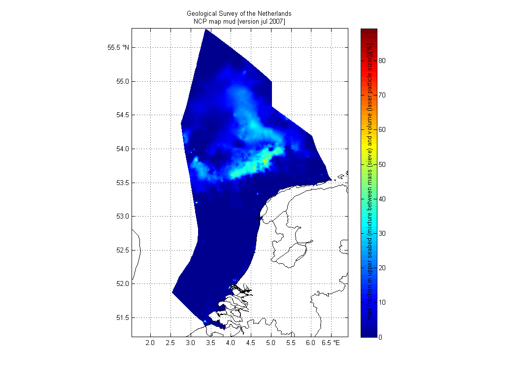
We used this image as Fig. 8 in our 2011 paper Mechanisms controlling the intra-annual mesoscale variability of SST and SPM in the southern North Sea.
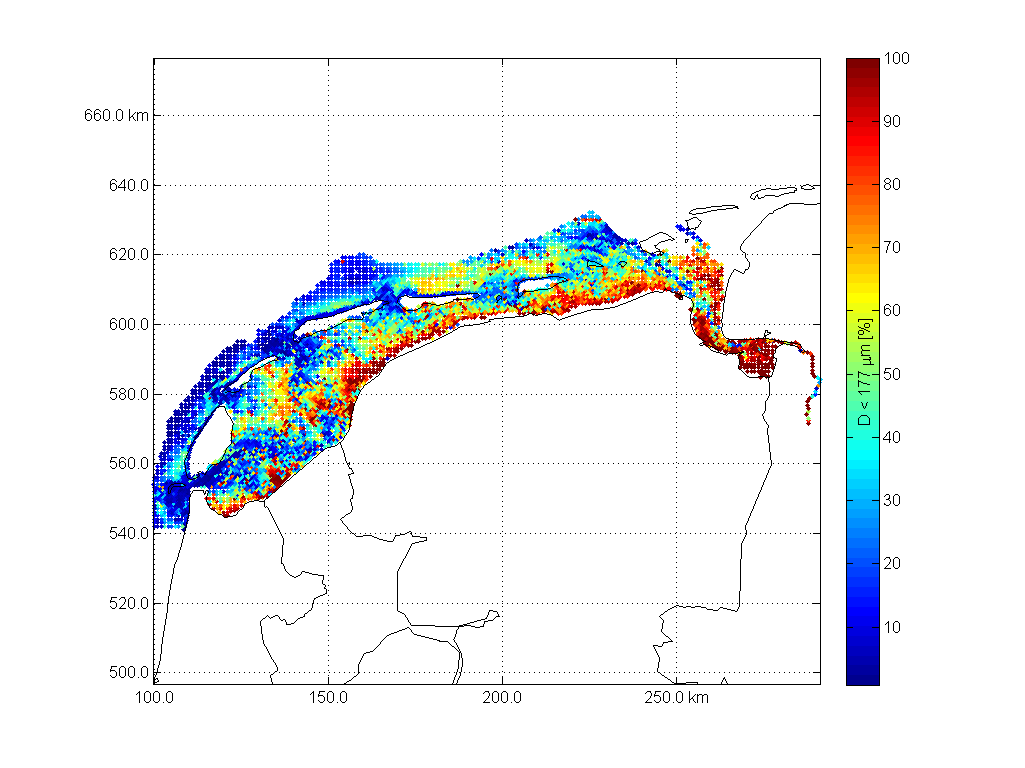
Sedimentatlas waddensea
A second Matlab example is a dataset used for Fig 9 in our 2008 paper Modeling large-scale cohesive sediment transport affected by small-scale biological activity. Here's an exmaple how to work with these data, find more script in
| Code Block |
|---|
 %oetsettings
%% load data
 F          = 'http://opendap.deltares.nl/thredds/dodsC/opendap/rijkswaterstaat/sedimentatlas_waddenzee/korrel.nc';
 D.lon      = ncread(F,'lon');
 D.lat      = ncread(F,'lat');
 D.cumphi   = ncread(F,'cumphi');
 D.diameter = ncread(F,'diameter');
[D.x,D.y]   = convertCoordinates(D.lon,D.lat,'CS1.code',4326,'CS2.code',28992);% wgs84 to RD
fraction = 10; % fraction to work with

%% add coastal data
L = nc2struct('http://opendap.deltares.nl/thredds/dodsC/opendap/deltares/landboundaries/northsea.nc')
[L.x,L.y]   = convertCoordinates(L.lon,L.lat,'CS1.code',4326,'CS2.code',28992);% wgs84 to RD

%% plot data
caxis            ([0 100])
scatter          (D.x,D.y,20,D.cumphi(fraction,:),'.')
colorbarwithvtext(['D < ',num2str(D.diameter(fraction)),' \mum [%]'])
axis equal
grid on
tickmap          ('xy')
axis(axis)
hold on
plot(L.x,L.y,'k')
box on
print2screensize(['sedimentatlas_waddenzee_fraction_',num2str(D.diameter(fraction)),'mm'])

%% plot in Google Earth
 KMLscatter(D.lat ,D.lon ,D.cumphi(10,:),'fileName',['sedimentatlas_waddenzee.kml'],...
    'CBcolorTitle',['D < ',num2str(D.diameter(fraction)),' \mum [%]'],...
 'CBcolorbarlocation',{'W'});
|