The best fit will be considered to be that one that gives the smallest deviation from the measured data. A loop over the previously created variable listCalibration will provide this information. Previously, the variables indicating the different properties around the best fit will be initialized to values that will certainly will be overwritten. Remember that the initial model set up could provide a better fit than any of the calibration simulation. So this case should also be included in the check loop. If the deviation of a case is smaller than the current one devBestFit, then that case should replace the current one (index, boundary condition used, roughness used, and deviation from the data).
indexBestFit = -1
bcBestFit = 1e100
roughnessBestFit = 1e100
devBestFit = 1e100
for i in range(1,len(timeSeriesToCompare)-1): # case 0 is data so don't use it.
    case = listCalibration[i-1]
    if case[2] < devBestFit:
        indexBestFit = i
        bcBestFit = case[0]
        roughnessBestFit = case[1]
        devBestFit = case[2]
Once the best fit has been found, you can print the corresponding values to the Messages console.
print "selected bc: " + str(bcBestFit) + "m3/s"
print "selected roughness " + str(roughnessBestFit) + "m^(1/3) s^-1"
Finally, the line corresponding to this best fit can be added to the chart using distinctive line color and width, and series name.
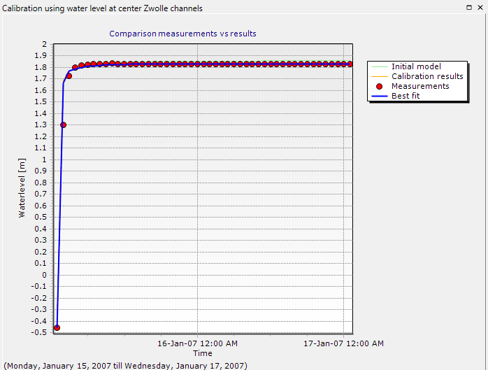
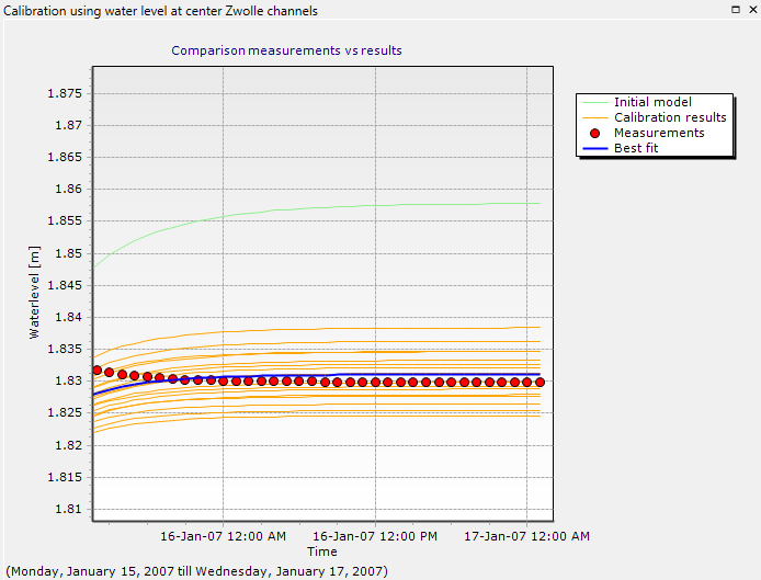
Or more in detail, if you zoom in (manually or with scripting):
Create a separate region for the the code of this section to keep your work tidy.
Export (calibration) results: Graphs, data and report