Page History

...

Note
Still to document TimeSpanComplexType

Table of Contents

Introduction

A list of pre-configured displays can be configured in the Display groups. When available on the file system, the name of the XML file is for example: DisplayGroups 1.00 default.xml

...

Figure 1 Example of time series display, showing two sub-plots and tree-view of pre-configured displays

Another option is to plot a longitudinal profile in the time series display (see figure 2). The main difference with the normal time series plot is, that on the X-axis the river chainage is plotted. With the control toolbar a specific time step can be selected.

...

Figure 2 Example of time series display, showing longitudinal profile.

The display groups are configured by first listing the names of the filters to be shown in the display (for example "Rain gauges", "Gauges" and "Fractions" in figure 3 below) under the displayGroup descriptor. The names of the subplots can then be added (e.g. "MacRitchie" and "Woodleigh" below). Each of the subplots is assigned a plotId which links to the definitions of the plots and the time series set to be used. For example in the Fractions displayGroup a stackPlot is defined with a max and min (this file is attached as an example). Please note that the colours, linestyle, precision etc are defined in the TimeSeriesDisplayConfig.

...

Root element for each displayGroup. A display group forms one of the main nodes in the tree view and may contain multiple displays. Multiple display groups may be defined.

Attributes:

description: Optional description
plot: Plot complex type
displayGroup: displayGroup complex type

...

Use the <area> element in combination with a <lineStyle> to obtain vertical lines.

Code Block

	xml
	xml


<subplot>
     <area>
        <lineStyle>solid</lineStyle>
        <lineWidth>10</lineWidth>
         <color>blue</color>
         <opaquenessPercentage>50</opaquenessPercentage>
           <timeSeriesSet>
                <moduleInstanceId>ImportMSW</moduleInstanceId>
                <valueType>scalar</valueType>
                <parameterId>Q.m</parameterId>
                <locationId>H-MS-LUIK</locationId>
                <locationId>H-MS-SINT</locationId>
                <timeSeriesType>external historical</timeSeriesType>
                <timeStep unit="hour"/>
                <relativeViewPeriod unit="day" start="-2" end="0"/>
                <readWriteMode>read only</readWriteMode>
           </timeSeriesSet>
        </area>
</subplot>

...

Below are two examples of a config and the resulting plot.

Code Block

	xml
	xml


		<subplot>
			<plotWeight>1</plotWeight>
			<line>
				<color>blue</color>
				<axis>left</axis>
				<timeSeriesSet>
					<moduleInstanceId>ImportTelemetry</moduleInstanceId>
					<valueType>scalar</valueType>
					<parameterId>H.obs</parameterId>
					<locationId>Hydro1</locationId>
					<timeSeriesType>external historical</timeSeriesType>
					<timeStep unit="minute" multiplier="15"/>
					<relativeViewPeriod unit="hour" start="-36" end="36"/>
					<readWriteMode>editing visible to all future task runs</readWriteMode>
				</timeSeriesSet>
			</line>
			<line>
				<color>blue</color>
				<axis>left</axis>
				<timeSeriesSet>
					<moduleInstanceId>ImportTelemetry</moduleInstanceId>
					<valueType>scalar</valueType>
					<parameterId>H.rated</parameterId>
					<locationId>Hydro3</locationId>
					<timeSeriesType>external historical</timeSeriesType>
					<timeStep unit="minute" multiplier="15"/>
					<relativeViewPeriod unit="hour" start="-36" end="36"/>
					<readWriteMode>editing visible to all future task runs</readWriteMode>
				</timeSeriesSet>
			</line>
			<line>
				<color>red</color>
				<axis>right</axis>
				<timeSeriesSet>
					<moduleInstanceId>ImportTelemetry</moduleInstanceId>
					<valueType>scalar</valueType>
					<parameterId>Q.obs</parameterId>
					<locationId>Hydro2</locationId>
					<timeSeriesType>external historical</timeSeriesType>
					<timeStep unit="minute" multiplier="15"/>
					<relativeViewPeriod unit="hour" start="-36" end="36"/>
					<readWriteMode>editing visible to all future task runs</readWriteMode>
				</timeSeriesSet>
			</line>
			<line>
				<color>red</color>
				<axis>right</axis>
				<timeSeriesSet>
					<moduleInstanceId>ImportTelemetry</moduleInstanceId>
					<valueType>scalar</valueType>
					<parameterId>Q.rated</parameterId>
					<locationId>Hydro4</locationId>
					<timeSeriesType>external historical</timeSeriesType>
					<timeStep unit="minute" multiplier="15"/>
					<relativeViewPeriod unit="hour" start="-36" end="36"/>
					<readWriteMode>editing visible to all future task runs</readWriteMode>
				</timeSeriesSet>
			</line>
		</subplot>

Code Block

	xml
	xml


		<subplot>
			<plotWeight>1</plotWeight>
			<line>
				<color>blue</color>
				<axis>right</axis>
				<timeSeriesSet>
					<moduleInstanceId>ImportTelemetry</moduleInstanceId>
					<valueType>scalar</valueType>
					<parameterId>H.obs</parameterId>
					<locationId>Hydro1</locationId>
					<timeSeriesType>external historical</timeSeriesType>
					<timeStep unit="minute" multiplier="15"/>
					<relativeViewPeriod unit="hour" start="-36" end="36"/>
					<readWriteMode>editing visible to all future task runs</readWriteMode>
				</timeSeriesSet>
			</line>
			<line>
				<color>red</color>
				<timeSeriesSet>
					<moduleInstanceId>ImportTelemetry</moduleInstanceId>
					<valueType>scalar</valueType>
					<parameterId>Q.obs</parameterId>
					<locationId>Hydro2</locationId>
					<timeSeriesType>external historical</timeSeriesType>
					<timeStep unit="minute" multiplier="15"/>
					<relativeViewPeriod unit="hour" start="-36" end="36"/>
					<readWriteMode>editing visible to all future task runs</readWriteMode>
				</timeSeriesSet>
			</line>
		</subplot>

Threshold line only for timeseries on the right y axis

...

Below an configuration and resulting plot

Code Block

	xml
	xml


<subplot>
			<line>
				<color>black</color>
				<lineStyle>none</lineStyle>
				<markerStyle>+</markerStyle>
				<markerSize>3</markerSize>
				<timeSeriesSet>
					<moduleInstanceId>ImportTelemetry</moduleInstanceId>
					<valueType>scalar</valueType>
					<parameterId>Q.rated</parameterId>
					<locationId>Hydro4</locationId>
					<timeSeriesType>external historical</timeSeriesType>
					<timeStep unit="minute" multiplier="15"/>
					<relativeViewPeriod unit="hour" start="-36" end="36"/>
					<readWriteMode>editing visible to all future task runs</readWriteMode>
				</timeSeriesSet>
			</line>
			<line>
				<color>black</color>
				<lineStyle>solid</lineStyle>
				<markerStyle>circle</markerStyle>
				<markerSize>6</markerSize>
				<axis>left</axis>
				<ratingAxis>
					<parameterGroupId>Water Level</parameterGroupId>
					<transformationType>dischargeStage</transformationType>
				</ratingAxis>
				<timeSeriesSet>
					<moduleInstanceId>ImportTelemetry</moduleInstanceId>
					<valueType>scalar</valueType>
					<parameterId>Q.obs</parameterId>
					<locationId>Hydro2</locationId>
					<timeSeriesType>external historical</timeSeriesType>
					<timeStep unit="minute" multiplier="15"/>
					<relativeViewPeriod unit="hour" start="-36" end="36"/>
					<readWriteMode>editing visible to all future task runs</readWriteMode>
				</timeSeriesSet>
			</line>
		</subplot>

...

currentSystemTime	view period x-axis (start-end)
12 Aug.2012	1 Oct.2011 - 30 Sept.2012
12 Sept.2012	1 Oct.2012 - 30 Sept.2013
12 Oct.2012	1 Oct.2012 - 30 Sept.2013

Code Block

	xml
	xml


<display name="SELI1 - Selway R nr Lowell - SWE">
	<startForwardLookingPeriod>--09-01</startForwardLookingPeriod>
	<season>
		<startMonthDay>--10-01</startMonthDay>
		<endMonthDay>--09-30</endMonthDay>
	</season>
	<locationId>SELI1L</locationId>
	<locationId>SELI1U</locationId>
	<plotId>SWE</plotId>
</display>

...

Options available when creating an area type display

AtrributesAttributes:

color: Overides other predefined colours
opaquenessPercentage: Opaqueness expressed as a percentage
IncludesZeros: When true the zero is always included in the painted extent

Note

Making stacked graphs

Since 2007/02 release the functionality of the SubPlotArea complex type has been extended to include stack plots. The only thing needed to implement this is to add a stackPlot="true" attribute to a subplot element. Attached to this page is a example of this funtionality.

If stackPlot is True, the timeseries of this subplot are plotted as stacked areas, except for the timeseries that are specified inside the (optional) element <area>. Area-series are always plotted as so called 'difference area'.

Attribute stackPlot is intended as overruling of the default series paint (i.e. line or bar)

It is not possible to combine 'stacked areas' and lines/bars in one plot.

A configuration example of an application of stacked graphs can be find in the how to page How to import and visualize rain and dropsize distribution data from WaterML 2.0 format.

VariableLineWidth

Options available when creating an variable line width type display

Image Added

Attributes:

markerColor: option to set marker color different from line color
lineWidthScaleFactor: factor to increase or decrease the line width
valueTimeSeriesSet: Time series for XY line plot
lineWidthTimeSeriesSet: Time series for line width of the XY plot lines

Example

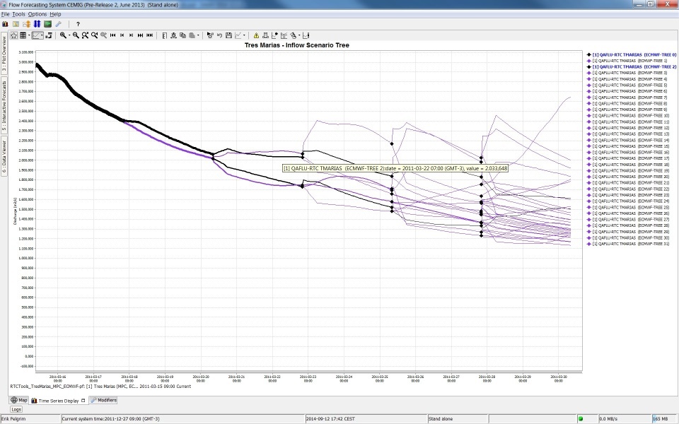
Below a screenshot of a variable line width plot for different ensemble members that have different line width's. In this case line width is an indication of the probability of the ensemble member. The sum of probability of all ensemble members at a time is one. Selecting separate ensemble members will mark them with the color black.

Image Added

Configuration used for above example

Code Block

language	xml
title	Example Configuration
collapse	true

	<displayGroup name="Scenario Tree Test">
		<display name="Tres Marias - Inflow Scenario Tree">
			<subplot>
				<variableLineWidth>
					<color>purple</color>
					<lineStyle>solid</lineStyle>
					<markerStyle>diamond</markerStyle>
					<markerSize>10</markerSize>
					<markerColor>black</markerColor>
					<lineWidthScaleFactor>10</lineWidthScaleFactor>
					<valueTimeSeriesSet>
						<moduleInstanceId>RTCTools_TresMarias_MPC_ECMWF-pf</moduleInstanceId>
						<valueType>scalar</valueType>
						<parameterId>QAFLU-RTC</parameterId>
						<locationId>TMARIAS</locationId>
						<timeSeriesType>simulated forecasting</timeSeriesType>
						<timeStep unit="hour" multiplier="1"/>
						<readWriteMode>read complete forecast</readWriteMode>
						<ensembleId>ECMWF-TREE</ensembleId>
					</valueTimeSeriesSet>
					<lineWidthTimeSeriesSet>
						<moduleInstanceId>RTCTools_TresMarias_MPC_ECMWF-pf</moduleInstanceId>
						<valueType>scalar</valueType>
						<parameterId>Probability</parameterId>
						<locationId>Probability</locationId>
						<timeSeriesType>simulated forecasting</timeSeriesType>
						<timeStep unit="hour" multiplier="1"/>
						<readWriteMode>read complete forecast</readWriteMode>
						<ensembleId>ECMWF-TREE</ensembleId>
					</lineWidthTimeSeriesSet>
				</variableLineWidth>
			</subplot>
		</display>
	</displayGroup>

Info
Display groups may be defined while DELFT-FEWS is running and reloaded by re-opening the time series dialogue. If a mistake is made, then the shortcuts item to open the tree view will not appear and an appropriate message will be generated. After resolving the mistake the item will again become available on re-loading the display.

Page tree

Versions Compared

Old Version 57

New Version 58

Key

Introduction

VariableLineWidth