...
The layout of the time series display is configured in an XML file in the System Configuration folder. When available on the file system, the name of the XML file is for example:
TimeSeriesDisplayConfig 1.00 default.xml
TimeSeriesDisplayConfig Fixed file name for the time series display settings1.00 Version number
default Flag to indicate the version is the default configuration (otherwise omitted).
Figure 13 shows the main elements of the TimeSeriesDisplay configuration. These are divided into a number of sections, each of which will be discussed individually (these are indicated with a + sign).
...
Time series statistical functions are statistical functions that use one equidistant, scalar time series to produce another one using a statistical function. When defined, a list of statistical functions will be displayed in the Time Series Display. If the user selects a function then for each (equidistant, scalar) time series in the display another one is generated and displayed with the calculated results. Calculated time series are displayed in the same graph as the time series they are based on. Check out the User Guide for visual details.
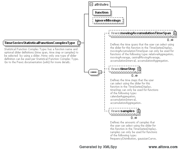
Some statistical functions require an additional accumulation time span, time step or samples which the user can select using a slider. As soon as the user selects a different value from the slider the calculation is launched with the new value.
The Statistical functions group defines dedicated graphing options shown in the combo box in the toolbar:
...
Accumulation aggregation (with associated time span or time step)
...
The accumulation interval sums the values for all time steps within the selected time window range. The time window range is defined by the associated time span or time step.
Attributes:
- function:
...
- accumulationAggregation
...
- movingAccumulationTimeSpan: Time
...
- spans that the user
...
- can select using the slider.
...
- or
- timeStep: Time steps that the user can select using the slider.
Accumulation interval (with associated time span or time step)
Creates an aggregation of a time series array. A relative time step is calculated by the selected time span and the start time of the period from the time series array.
Attributes:
- function: relativeAggregation
- movingAccumulationTimeSpan: Time spans that the user selects by using the slider.
Duration exceedence
Sorts the values in a time series array and its flags in descending order.
Attributes:
- function: durationExceedence
- ignoreMissings: when true, missing values are ignored and each duration will be calculated from the available values within the current time window.
When false, missing values are added to the end of the sorted series.
Duration non-exceedence
...
The accumulation interval function creates cumulative series for several intervals. For the first output time step in each interval the output value equals the input value for that time step. For a given other output time step the output value is equal to the sum of the input value for that time step and the previous output value. The intervals are defined by the selected time span or the selected time step. If a time span is selected, then the function uses the time span as the size for the intervals and the first interval starts at the start of the period that is visible in the time series display. If a time step is selected, then the function uses the selected time step to create intervals. Each period between two consecutive time steps in the selected time step is an interval.
Attributes:
- function:
...
- accumulationInterval
...
- movingAccumulationTimeSpan: Time spans that the user can select using the slider.
or - timeStep: Time steps that the user can select using the slider.
Boxplot
The data is graphically displayed by a box-and-whisker diagram. The following five-number summaries are displayed: the smallest observation (sample minimum), lower quartile (Q1), median (Q2), upper quartile (Q3), and largest observation (sample maximum). An additional dot is plotted to represent the mean of the data in addition to the median.
Attributes:
- function: boxPlot
Note: The displayed diagram is no longer a graph of unit time and therefore uses a different panel for displaying the graph. The associated table panel is currently not working for this type of graph and therefore the table toggle button will be disabled.
Calendar aggregation (with associated time step)
Creates an aggregation of a time series array according to the selected time step.
Attributes:
- function: calendarAggregation
- timeStep: Time steps
Moving average (with associated time span)
A moving average calculates the mean value of the all values within the selected time window.
Attributes:
- function: movingAverage
- ignoreMissings: when true, missing values are ignored and each average will be calculated from the available values within the current time window.
When false, calculated values will be set to missing if one or more values within the current time window are missing. - movingAccumulationTimeSpan: Time spans that the user selects by using the slider.
...
Central moving average
...
(
...
with associated time span)
A central moving average calculates the mean value of the time window of which the current value is in the middle. It is the same as the moving average, but shifted to the past for half the time window.
Attributes:
- function: centralMovingAverage
- ignoreMissings: when true, missing values are ignored and each average will be calculated from the available values within the current time window.
When false, calculated values will be set to missing if one or more values within the current time window are missing. - movingAccumulationTimeSpan: Time spans that the user selects by using the slider.
The central moving average function only works for true equidistant data (i.e. no daysOfMonths etc.)
The difference between moving average and central moving average is that the central moving average uses values before and after the current value to calculate the average. Moving average only uses values in the past.
Accumulation interval (with associated time span or time step)
...
Cumulative
Creates a continuous accumulation over entire timeseries.
Attributes:
- function: cumulative
Differences
Shows the difference against a reference level or a series. If using a series, the oldest series (creation time) is taken as reference by default
Attributes:
- function: differences
Double Mass Curve
Plots two series on differnt axis to study consistency and trends
Attributes:
- function:
...
- doubleMassCurve
Duration exceedence
Sorts the values in a time series array and its flags in descending order.
Attributes:
- function: durationExceedence
- ignoreMissings: when true, missing values are ignored and each duration will be calculated from the available values within the current time window.
When false, missing values are added to the end of the sorted series.
Duration non-exceedence
Sorts the values in a time series array and its flags in ascending order
Accumulation aggregation (with associated time span or time step)
The accumulation interval sums the values for all time steps within the selected time window range. The time window range is defined by the associated time span or time step.
Attributes:
- function: accumulationAggregationdurationNonExceedence
- movingAccumulationTimeSpan: Time spans that the user can select using the slider.
or timeStep: Time steps that the user can select using the slider. - ignoreMissings: when true, missing values are ignored and each duration will be calculated from the available values within the current time window.
When false, missing values are added to the end of the sorted series.
Elevation
Show parameter values against the elevation of the location on one particular time. The time for which the values are shown can be altered with a slider bar
Attributes:
- function: elevation
Ensemble percentile exceedence
Plots for the selected time stamp(s) each member of an ensemble along the horzontal axis, sorted by value.
Attributes:
- function: ensemblePercentileExceedence
Frequency distribution (with associated samples)
The frequencies of the available values are counted and are plotted within a number of bins to create a frequency distribution. The number of bins can be selected using the slider. The data range that is covered by the bins can be changed as follows. Clicking the "Set boundaries" button brings up the "Set boundaries" dialog. In this dialog the lowest bin boundary and the highest bin boundary can be changed. The space between these two boundaries is divided regularly into the selected number of bins. Initially the boundaries are in automatic mode. In automatic mode for each time series the minimum data value and the maximum data value are used as boundaries. When the user selects new boundaries manually, then the new boundaries will be used instead, i.e. manual mode. In manual mode the boundaries are fixed and the same boundaries are used for all time series, until they are changed again. This makes comparisons between different time series possible. When the user clicks the "Automatic" button, then the boundaries will be in automatic mode again.
In manual mode the selected boundaries are remembered. This means that when the user closes and re-opens the time series display or starts working in another separate time series display, then in manual mode the previously selected boundaries will still be used for new frequency distributions. The mode will also be the same for all time series displays.
Attributes:
- function: frequencyDistribution
- samples: The number of bins that the user can select using the slider.
Gaussian curve (with associated samples)
The mean value and standard deviation are calculated for the timeseries from which the normal distribution function is calculated. The selected sample determines in how many samples the normal distribution function is divided into.
Attributes:
- function: gaussianCurve
- samples: Definition of samples sizes that the user selects by using the slider.
Note: The displayed diagram is no longer a graph of unit time and therefore uses a different panel for displaying the graph. The associated table panel is currently not working for this type of graph and therefore the table toggle button will be disabled.
Show peaks above value
A scatterplot is made where the x-axis shows the duration of a 'peak' (=values within this peak-area are all above the given reference level), the y-axis shows the normalized difference between the parameter value and the reference level. The reference level can be altered by entering a value into the input field associated with this statistical function. After clicking 'Apply' the result time series array is returned.
If no reference level is entered, then the 'peak' areas are determined according to the minimum available value of the input time series array.
Attributes:
- function: showPeaksAbove
- label: label used in the combobox to select a statistical function (since 2015.01).
Subelements:
- season (since 2015.01): one ore more color seasons can be configured with a color that will be used to display a point if the time of the show peaks above plot point is in that period. Periods should NOT be overlapping.
Historical analysis
Allows comparison of the current situation with selected previous years at the same moment (seasonal selection) within the year.
Attributes:
- function: historicalAnalysis
- historicalPeriods: Definition of season as well as the moment when the display should look forward instead of backward to plot the coming season
| Code Block | ||
|---|---|---|
| ||
   <historicalPeriods>
    <historicalPeriod>
     <startForwardLookingPeriod>--04-01</startForwardLookingPeriod>
     <season startMonthDay="--04-01" endMonthDay="--10-01" label="zomer"/>
    </historicalPeriod>
</historicalPeriods> |
Historical scatter plot
Shows the scatter plot, allows subselection by season and year
Attributes:
- function: historicalScatterPlot
- historicalPeriods: Definition of season as well as the moment when the display should look forward instead of backward to plot the coming season
Historical show lows below
Shows the lows below a entered value, allows subselection by year and season
Attributes:
- function: historicalShowLowsBelow
- historicalPeriods: Definition of season as well as the moment when the display should look forward instead of backward to plot the coming season
Historical show peaks above
Shows the peaks above a entered value, allows subselection by year and season
Attributes:
- function: historicalShowPeaksAbove
- historicalPeriods: Definition of season as well as the moment when the display should look forward instead of backward to plot the coming season
Moving average (with associated time span)
A moving average calculates the mean value of the all values within the selected time window.
Attributes:
- function: movingAverage
- ignoreMissings: when true, missing values are ignored and each average will be calculated from the available values within the current time window.
When false, calculated values will be set to missing if one or more values within the current time window are missing. - movingAccumulationTimeSpan: Time spans that the user selects by using the slider.
The moving average function only works for true equidistant data (i.e. no daysOfMonths etc.)
The difference between moving average and central moving average is that the central moving average uses values before and after the current value to calculate the average. Moving average only uses values in the past.
Normalized Flow
Function to convert flowrate (e.g. in m3/s) to volume/time/area (e.g. l/s/ha) using area function
Attributes:
- function: normalizedFlow
- label: caption used in function selection
- ignoreMissings: when true, missing values are ignored and each average will be calculated from the available values within the current time window.
When false, calculated values will be set to missing if one or more values within the current time window are missing. - areaFunction: attribute aware function to transfer input parameter series
- parameterId: parameter used for unit in display
- allowedInputParameterId: series to be converted using area function
| Code Block | ||
|---|---|---|
| ||
<statisticalFunction function="normalizedFlow" label="Flow (mm/day)" ignoreMissings="true">
  <areaFunction>@AREA_HA@*10/86400</areaFunction>
  <parameterId>Q.mmd</parameterId>
  <allowedInputParameterId>Q.obs</allowedInputParameterId>
</statisticalFunction> |
Principle Component Analysis
The Principal Component Analysis function uses independent historical data (observations) and dependent data (e.g. a simulated basin value) to compute a number of regression equations using the Principal Component Analysis technique. The resulting equation is applied with current observations to estimate the current basin value.
Attributes:
- function: principalcomponentanalysis
- observedParameterId: parameter referencing the independent (observed) series
- simulatedParameterId: parameter referencing the dependent (simulated) series
- dateFormat: optional
| Code Block |
|---|
<statisticalFunction function="principalcomponentanalysis">
   <observedParameterId>SWE.m</observedParameterId>
   <simulatedParameterId>SWE.sim</simulatedParameterId>
   <dateFormat>MM-dd-yyyy</dateFormat>
</statisticalFunction> |
Principal Component Analysis Jack Knife
Same as principal component analysis, using the Jack Knife technique
Attributes:
- function: principalcomponentanalysisJackKnife
- observedParameterId: parameter referencing the independent (observed) series
- simulatedParameterId: parameter referencing the dependent (simulated) series
- dateFormat: optional
Relative aggregation (with associated time span)
Creates an aggregation of a time series array. A relative time step is calculated by the selected time span and the start time of the period from the time series array.
Attributes:
- function: relativeAggregation
- movingAccumulationTimeSpan: Time spans that the user selects by using the slider.
Scatter plot
Creates a scatter plot of two selected series
Attributes:
- function: scatterPlot
Show lows below value
A scatterplot is made where the x-axis shows the duration of a 'low' (=values within this low-area are all beneath the given reference level), the y-axis shows the normalized difference between the parameter value and the reference level. The reference level can be altered by entering a value into the input field associated with this statistical function. After clicking 'Apply' the result time series array is returned.
If no reference level is entered, then the 'low' areas are determined according to the maximum available value of the input time series array.
Attributes:
- function: showLowsBelow
See "show peaks above" for label and season functionality.
Show peaks above value
A scatterplot is made where the x-axis shows the duration of a 'peak' (=values within this peak-area are all above the given reference level), the y-axis shows the normalized difference between the parameter value and the reference level. The reference level can be altered by entering a value into the input field associated with this statistical function. After clicking 'Apply' the result time series array is returned.
If no reference level is entered, then the 'peak' areas are determined according to the minimum available value of the input time series array.
Attributes:
- function: showPeaksAbove
- label: label used in the combobox to select a statistical function (since 2015.01).
Subelements:
- season (since 2015.01): one ore more color seasons can be configured with a color that will be used to display a point if the time of the show peaks above plot point is in that period. Periods should NOT be overlapping.
| Code Block | ||||
|---|---|---|---|---|
| ||||
<statisticalFunction function="showPeaksAbove" label="Seasonal Show Peaks Above">
<season startMonthDay="--01 | ||||
| Code Block | ||||
| xml | xml | <statisticalFunction function="showPeaksAbove" label="Seasonal Show Peaks Above"> <season startMonthDay="--01-01" endMonthDay="--03-31" label="January,February,March" color="orange"/> <season startMonthDay="--04-01" endMonthDay="--06-30" label="April, May, June" color="green"/> <season startMonthDay="--07-01" endMonthDay="--0903-3031" label="JulyJanuary, AugustFebruary, SeptemberMarch" color="yelloworange"/> <season startMonthDay="--1004-01" endMonthDay="--1206-3130" label="OctoberApril, NovemberMay, DecemberJune" color="redgreen"/> </statisticalFunction> |
Show lows below value
A scatterplot is made where the x-axis shows the duration of a 'low' (=values within this low-area are all beneath the given reference level), the y-axis shows the normalized difference between the parameter value and the reference level. The reference level can be altered by entering a value into the input field associated with this statistical function. After clicking 'Apply' the result time series array is returned.
If no reference level is entered, then the 'low' areas are determined according to the maximum available value of the input time series array.
Attributes:
- function: showLowsBelow
See "show peaks above" for label and season functionality.
Scatterplot
The data is displayed as a collection of points, each having the value of the timeseries determining the position on the horizontal axis and the value of the other timeseries (one or more) determining the position on the vertical axis.
The timeseries used for the horizontal- and vertical axis can be changed by the user by using the 'Series selection' dialog, which is opened by clicking on the 'Edit' button. Note: The displayed diagram is no longer a graph of unit time and therefore uses a different panel for displaying the graph. The associated table panel is currently not working for this type of graph and therefore the table toggle button will be disabled.
Attributes:
function: scatterPlot
See "show peaks above" for label and season functionality.
Boxplot
The data is graphically displayed by a box-and-whisker diagram. The following five-number summaries are displayed: the smallest observation (sample minimum), lower quartile (Q1), median (Q2), upper quartile (Q3), and largest observation (sample maximum). An additional dot is plotted to represent the mean of the data in addition to the median.
Attributes:
- function: boxPlot
	<season startMonthDay="--07-01" endMonthDay="--09-30" label="July, August, September" color="yellow"/>
	<season startMonthDay="--10-01" endMonthDay="--12-31" label="October, November, December" color="red"/>
</statisticalFunction> |
Scatterplot
The data is displayed as a collection of points, each having the value of the timeseries determining the position on the horizontal axis and the value of the other timeseries (one or more) determining the position on the vertical axis.
The timeseries used for the horizontal- and vertical axis can be changed by the user by using the 'Series selection' dialog, which is opened by clicking on the 'Edit' button. NoteNote: The displayed diagram is no longer a graph of unit time and therefore uses a different panel for displaying the graph. The associated table panel is currently not working for this type of graph and therefore the table toggle button will be disabled.
Attributes:
function: scatterPlot
See "show peaks above" for label and season functionality.
Schemas for the slider
movingAccumulationTimeSpan
...