...
Therefore, eCoDeS requires loading or defining a spatially varying bathymetry (either loaded as raster or point cloud data) in generic data. Find more information here.
Note: point-clouds with large amounts of points (>10.000 points) can be slow due to computational time.
An example of a loaded point cloud bathymetry of the Western Scheld region is shown below.

2. Load/create a species and associated response curves
...
In the table below, the recalculated response is shown for submerged vegetation, calculated with the values from the Ecological knowledge base of HABITAT, combined with a default water extinction coefficient k=1.

After pressing “keep changes”, the response curve is stored (also on your PC for later use) and you can close the response curve panel by clicking on the "X".
...
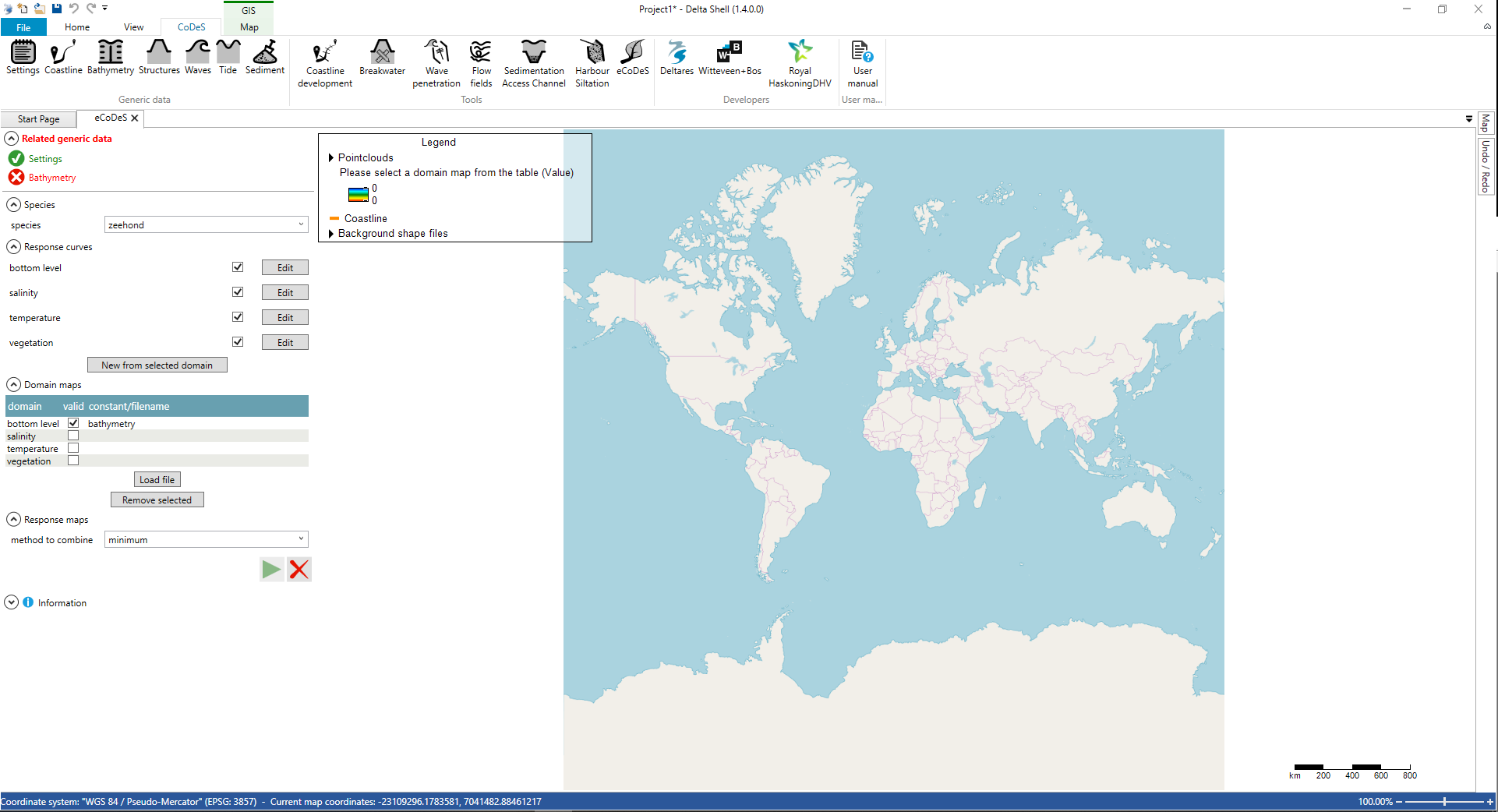
After pressing the calculate button the following screen appears:

The response map associated with submerged vegetation (considering water depth) is now shown on the map and appears under the “domain maps” panel.
...
Next, make a new species by typing “Otter” in the species panel. Now you can edit the response curves for “Otter” for domain maps “bottom level” and “submerged vegetation - bottom level” using the information in the Ecological Knowledge Base for the Otter, see the Figure below.

After creating the Otter and its response curves, the new HSI response map can be calculated using the calculate (play) button.
...
When using the “minimum” method, the results as presented in the Figure below are obtained for “Otter”.

Examples
No example is available (yet).
...