...
- unit identifies the time unit with which the time span is defined (enumeration of second, minute, hour, day, week).
- start identifies the start time of the time span with reference to the T0 (in multiples of the unit defined).
- end identifies the start time of the time span with reference to the T0 (in multiples of the unit defined).
Scroller default view period
The optional scrollerDefaultViewPeriod can be used to define the time span of data displayed in the long term scroller of the time series display (unless overruled by the user).
showAllScrollerData
When true the long term scroller always show the full period where the time series in the scroller have data. This can be configured instead of <scrollerDefaultViewPeriod> and is available since 2023.02.
| Anchor | ||||
|---|---|---|---|---|
|
...
- %LOCATION_ID%
- %LOCATION_NAME%
- %LOCATION_SHORTNAME%
- %LOCATION_DESCRIPTION%
- %PARAMETER_ID%
- %PARAMETER_NAME%
- %PARAMETER_SHORTNAME%
- %PARAMETER_DESCRIPTION%
- %PARAMETER_UNIT%
- %QUALIFIER_NAME%
- %MODULE_INSTANCE_ID%
- %MODULE_INSTANCE_NAME%
- %MODULE_INSTANCE_DESCRIPTION%
Time Markers Display Configuration
Time series display markers are informative lines in the display. These may be defined to display vertical lines for times of interest. The configuration of horizontal lines for thresholds and the zero baseline is also included in this definition. Markers can be defined for four time values as well as for the thresholds and the zero baseline. Vertical lines are also available as lineStyle for plotting of time series, see below.
for time series
Class Breaks
Class breaks (map legend) is used in the spatial plots and vertical profiles. The classbreaks can be configured in the Spatial Display configuration, but also in the TimeSeriesDisplayConfig file. When calssbreaks are added in this file, it requires a classbreak Id. The classBreak Id can then be used in the Spatial Display or Display Groups.
| Code Block |
|---|
    <classBreaks>
        <classBreaks id="rainfall_forecasts">
            <description>Rainfall Forecasts</description>
            <unitVisible>true</unitVisible>
            <break color="FFFFFF" lowerValue="0" opaquenessPercentage="35"/>
            <break color="99E9FF" lowerValue="0.2" opaquenessPercentage="35"/>
            <break color="00C8FF" lowerValue="1" opaquenessPercentage="60"/>
            <break color="0053FF" lowerValue="5" opaquenessPercentage="60"/>
            <break color="00956A" lowerValue="10" opaquenessPercentage="60"/>
            <break color="00FA10" lowerValue="25" opaquenessPercentage="60"/>
            <break color="F5F50A" lowerValue="50" opaquenessPercentage="60"/>
            <break color="FF9600" lowerValue="75" opaquenessPercentage="60"/>
            <break color="FF0000" lowerValue="100" opaquenessPercentage="80"/>
            <break color="960000" lowerValue="200" opaquenessPercentage="80"/>
            <break color="FF00CC" lowerValue="400" opaquenessPercentage="80"/>
        </classBreaks>
</classBreaks> |
Time Markers Display Configuration
Time series display markers are informative lines in the display. These may be defined to display vertical lines for times of interest. The configuration of horizontal lines for thresholds and the zero baseline is also included in this definition. Markers can be defined for four time values as well as for the thresholds and the zero baseline. Vertical lines are also available as lineStyle for plotting of time series, see below.
for time series
- systemTime
- displayTime: time that can be set with the display time button (clock icon) in the time series dialog, by default equals the system time
- timeZero: T0 of the external forecast time series
- forecastStartTime (since stable build 2014.01). This will show vertical lines in charts for the start times of forecast time series, i.e. time series of type external forecasting, simulated forecasting. It will only be shown when the forecast time series is configured with "read complete forecast" as readWriteMode.
- threshold
- zeroBaseline
timeOfValidity (since 2016.01). This marker should be visualized in the display when the Tv button is activated. This will show vertical lines in charts placed at the Time of Validity (Tv) of that display node. The Tv is determined using the timeOfValiditySearchPeriod. The functionality of Time of Validity is more exhaustively described in the Validation Status page.Anchor timeSeriesDisplayConfig_TimeMarkersDisplayConfiguration timeSeriesDisplayConfig_TimeMarkersDisplayConfiguration
...
Since 2021.01 it is possible to a just adjust the default colors. A A default color is used when no color is configured for a a series or to prevent duplicate colors for non-predefined plots. The colors are used in the order as configured. The list below is used when no default colors are configured.
...
Note: The displayed diagram is no longer a graph of unit time and therefore uses a different panel for displaying the graph. The associated table panel is currently not working for this type of graph and therefore the table toggle button will be disabled.
Historical analysis
...
table panel is currently not working for this type of graph and therefore the table toggle button will be disabled.
Historical analysis
Allows comparison of the current situation with selected previous years at the same moment (seasonal selection) within the year.
Attributes:
- function: historicalAnalysis
- historicalPeriods: Definition of season as well as the moment when the display should look forward instead of backward to plot the coming season
| Code Block | ||||
|---|---|---|---|---|
| ||||
   <historicalPeriods>
    <historicalPeriod>
     <startForwardLookingPeriod>--04-01</startForwardLookingPeriod>
     <season startMonthDay="--04-01" endMonthDay="--10-01" label="zomer"/>
    </historicalPeriod>
</historicalPeriods> |
Historical scatter plot
Shows the scatter plot, allows subselection by season and year
Attributes:
- function: historicalAnalysishistoricalScatterPlot
- historicalPeriodsseason: Definition of season as well as the moment when the display should look forward instead of backward to plot the coming seasonseasons
| Code Block | ||||
|---|---|---|---|---|
| ||||
<historicalPeriods> <historicalPeriod> <startForwardLookingPeriod>--04-01</startForwardLookingPeriod> <statisticalFunction function="historicalShowPeaksAbove"> <season startMonthDay="--01-01" endMonthDay="--12-31" label="Year" color="black"/> <season startMonthDay="--04-01" endMonthDay="--1009-0130" label="zomerGrow Season" color="gray"/> </historicalPeriod> </historicalPeriods> |
Historical scatter plot
Shows the scatter plot, allows subselection by season and year
Attributes:
- function: historicalScatterPlot
- season: Definition of seasons
| Code Block | ||||
|---|---|---|---|---|
| ||||
<statisticalFunction function="historicalShowPeaksAbove">
	<season startMonthDay="--01-01" endMonthDay="--12-31" label="Year" color="black"/>
	<season startMonthDay="--04-01" endMonthDay="--09-30" label="Grow Season" color="gray"/>
</statisticalFunction> |
Historical show lows below
Shows the lows below a entered value, allows subselection by year and season
Attributes:
- function: historicalShowLowsBelow
- season: Definition of seasons
Historical show peaks above
Shows the peaks above a entered value, allows subselection by year and season
Attributes:
- function: historicalShowPeaksAbove
- season: Definition of seasons
Moving average (with associated time span)
A moving average calculates the mean value of the all values within the selected time window.
Attributes:
- function: movingAverage
- ignoreMissings: when true, missing values are ignored and each average will be calculated from the available values within the current time window.
When false, calculated values will be set to missing if one or more values within the current time window are missing. - movingAccumulationTimeSpan: Time spans that the user selects by using the slider.
The moving average function only works for true equidistant data (i.e. no daysOfMonths etc.)
The difference between moving average and central moving average is that the central moving average uses values before and after the current value to calculate the average. Moving average only uses values in the past.
Normalized Flow
Function to convert flowrate (e.g. in m3/s) to volume/time/area (e.g. l/s/ha) using area function
Attributes:
...
</statisticalFunction> |
Historical show lows below
Shows the lows below a entered value, allows subselection by year and season
Attributes:
- function: historicalShowLowsBelow
- season: Definition of seasons
Historical show peaks above
Shows the peaks above a entered value, allows subselection by year and season
Attributes:
- function: historicalShowPeaksAbove
- season: Definition of seasons
Moving average (with associated time span)
A moving average calculates the mean value of the all values within the selected time window.
Attributes:
- function: movingAverage
- ignoreMissings: when true, missing values are ignored and each average will be calculated from the available values within the current time window.
When false, calculated values will be set to missing if one or more values within the current time window are missing. - movingAccumulationTimeSpan: Time spans that the user selects by using the slider.
The moving average function only works for true equidistant data (i.e. no daysOfMonths etc.)
The difference between moving average and central moving average is that the central moving average uses values before and after the current value to calculate the average. Moving average only uses values in the past.
Normalized Flow
Function to convert flowrate (e.g. in m3/s) to volume/time/area (e.g. l/s/ha) using area function
Attributes:
- function: normalizedFlow
- label: caption used in function selection
- ignoreMissings: when true, missing values are ignored and each average will be calculated from the available values within the current time window.
When false, calculated values will be set to missing if one or more values within the current time window are missing. - areaFunction: attribute aware function to transfer input parameter series
- parameterId: parameter used for unit in display
- allowedInputParameterId: series to be converted using area function
| Code Block | ||||
|---|---|---|---|---|
| ||||
<statisticalFunction function="normalizedFlow" label="Flow (mm/day)" ignoreMissings="true">
  <areaFunction>@AREA_HA@*10/86400</areaFunction>
  <parameterId>Q.mmd</parameterId>
  <allowedInputParameterId>Q.obs</allowedInputParameterId>
</statisticalFunction> |
Principle Component Analysis
The Principal Component Analysis function uses independent historical data (observations) and dependent data (e.g. a simulated basin value) to compute a number of regression equations using the Principal Component Analysis technique. The resulting equation is applied with current observations to estimate the current basin value.
Attributes:
- function: principalcomponentanalysis
- observedParameterId: parameter referencing the independent (observed) series
- simulatedParameterId: parameter referencing the dependent (simulated) series
- dateFormat: optional
| Code Block | ||
|---|---|---|
| ||
<statisticalFunction function="principalcomponentanalysis">
   <observedParameterId>SWE.m</observedParameterId>
   <simulatedParameterId>SWE.sim</simulatedParameterId>
   <dateFormat>MM-dd-yyyy</dateFormat>
</statisticalFunction> |
Principal Component Analysis Jack Knife
Same as principal component analysis, using the Jack Knife technique
Attributes:
- function: principalcomponentanalysisJackKnife
- observedParameterId: parameter referencing the independent (observed) series
- simulatedParameterId: parameter referencing the dependent (simulated) series
- dateFormat: optional
Relative aggregation (with associated time span)
Creates an aggregation of a time series array. A relative time step is calculated by the selected time span and the start time of the period from the time series array.
Attributes:
- function: relativeAggregation
- movingAccumulationTimeSpan: Time spans that the user selects by using the slider.
Scatter plot
Creates a scatter plot of two selected series
Attributes:
- function: scatterPlot
Show lows below value
A scatterplot is made where the x-axis shows the duration of a 'low' (=values within this low-area are all beneath the given reference level), the y-axis shows the normalized difference between the parameter value and the reference level. The reference level can be altered by entering a value into the input field associated with this statistical function. After clicking 'Apply' the result time series array is returned.
If no reference level is entered, then the 'low' areas are determined according to the maximum available value of the input time series array.
Attributes:
- function: showLowsBelow
See "show peaks above" for label and season functionality.
Show peaks above value
A scatterplot is made where the x-axis shows the duration of a 'peak' (=values within this peak-area are all above the given reference level), the y-axis shows the normalized difference between the parameter value and the reference level. The reference level can be altered by entering a value into the input field associated with this statistical function. After clicking 'Apply' the result time series array is returned.
If no reference level is entered, then the 'peak' areas are determined according to the minimum available value of the input time series array.
Attributes:
- function: showPeaksAbove
- label: label used in the combobox to select a statistical function (since 2015.01).
Subelements:
- season (since 2015.01): one ore more color seasons can be configured with a color that will be used to display a point if the time of the show peaks above plot point is in that period. Periods should NOT be overlapping.
| Code Block | ||||
|---|---|---|---|---|
| ||||
<statisticalFunction function="showPeaksAbove" label="Seasonal Show Peaks Above">
	<season startMonthDay="--01-01" endMonthDay="--03-31" label="January,February,March" color="orange"/>
	<season startMonthDay="--04-01" endMonthDay="--06-30" label="April, May, June" color="green"/>
	<season startMonthDay="--07-01" endMonthDay="--09-30" label="July, August, September" color="yellow"/>
	<season startMonthDay="--10-01" endMonthDay="--12-31" label="October, November, December" color="red"/>
</statisticalFunction> |
Scatterplot
The data is displayed as a collection of points, each having the value of the timeseries determining the position on the horizontal axis and the value of the other timeseries (one or more) determining the position on the vertical axis.
The timeseries used for the horizontal- and vertical axis can be changed by the user by using the 'Series selection' dialog, which is opened by clicking on the 'Edit' button. Note: The displayed diagram is no longer a graph of unit time and therefore uses a different panel for displaying the graph. The associated table panel is currently not working for this type of graph and therefore the table toggle button will be disabled.
Attributes:
function: scatterPlot
See "show peaks above" for label and season functionality.
Schemas for the slider
movingAccumulationTimeSpan
Defines the time spans that the user can select using the slider for this function in the TimeSeriesDisplay. MovingAccumulationTimeSpan can only be used for functions of the following type: relativeAggregation, movingAverage, centralMovingAverage, accumulationInterval, accumulationAggregation.
timeStep
Defines the time steps that the user can select using the slider for this function in the TimeSeriesDisplay. TimeStep can only be used for functions of the following type: calendarAggregation, accumulationInterval, accumulationAggregation.
samples
Defines the amounts of samples that the user can select using the slider for this function in the TimeSeriesDisplay. Samples can only be used for functions of the following type: frequencyDistribution, gaussianCurve.
quickViewStatisticalFunction
Through the quickViewStatisticalFunction you can define a shortcut key (with optional icon) at the toolbar to a statistical function.
LongTermPeriodic
This function adds periodic time series based on the long term scroller (see highlighted in red).
This can be used to compare values of time series compared to what is “normal” on that date of different years.
Multiple different statistic types can be configured within this function, for each type a time series is added.
The statistics wil be calculated based on all values on the same day of the years, for all years included in the whole period of the long term scroller.
For this the long term scroller should be visible.
This is especially designed for time series with a daily time step.
| Code Block | ||||
|---|---|---|---|---|
| ||||
<statisticalFunction function="longTermPeriodic" label="Long Term Periodic" ignoreMissings="true">
	<statisticType type="MIN" label="Minimum"/>
	<statisticType type="MAX" label="Maximum"/>
	<statisticType type="PERCENTILEEXCEEDENCE" value="50" label="50 percentiel"/>
</statisticalFunction> |

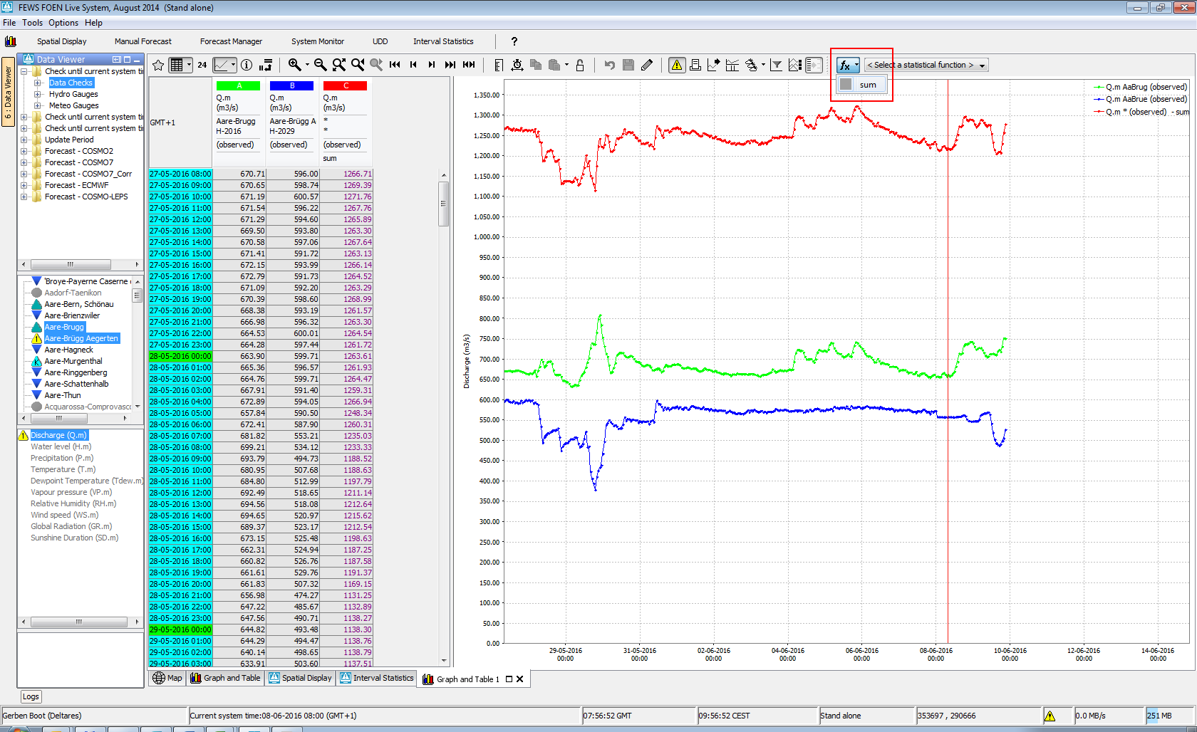
combinedTimeSeriesStatisticalFunctions
This option add a new timeseries to a plot which is the result of a statistical operation based the available timeseries in that plot. It will be filtered per parameter. E.g. if you have 4 waterlevel timeseries of 4 different gauges and you select the MAX statisticType, a new timeseries with the maximum value (per timestep) of those 4 gauges will be plotted
...
| Code Block | ||||
|---|---|---|---|---|
| ||||
<statisticalFunction function="normalizedFlow" label="Flow (mm/day)" ignoreMissings="true">
  <areaFunction>@AREA_HA@*10/86400</areaFunction>
  <parameterId>Q.mmd</parameterId>
  <allowedInputParameterId>Q.obs</allowedInputParameterId>
</statisticalFunction> |
Principle Component Analysis
The Principal Component Analysis function uses independent historical data (observations) and dependent data (e.g. a simulated basin value) to compute a number of regression equations using the Principal Component Analysis technique. The resulting equation is applied with current observations to estimate the current basin value.
Attributes:
- function: principalcomponentanalysis
- observedParameterId: parameter referencing the independent (observed) series
- simulatedParameterId: parameter referencing the dependent (simulated) series
- dateFormat: optional
| Code Block | ||
|---|---|---|
| ||
<statisticalFunction function="principalcomponentanalysis">
   <observedParameterId>SWE.m</observedParameterId>
   <simulatedParameterId>SWE.sim</simulatedParameterId>
   <dateFormat>MM-dd-yyyy</dateFormat>
</statisticalFunction> |
Principal Component Analysis Jack Knife
Same as principal component analysis, using the Jack Knife technique
Attributes:
- function: principalcomponentanalysisJackKnife
- observedParameterId: parameter referencing the independent (observed) series
- simulatedParameterId: parameter referencing the dependent (simulated) series
- dateFormat: optional
Relative aggregation (with associated time span)
Creates an aggregation of a time series array. A relative time step is calculated by the selected time span and the start time of the period from the time series array.
Attributes:
- function: relativeAggregation
- movingAccumulationTimeSpan: Time spans that the user selects by using the slider.
Scatter plot
Creates a scatter plot of two selected series
Attributes:
- function: scatterPlot
Show lows below value
A scatterplot is made where the x-axis shows the duration of a 'low' (=values within this low-area are all beneath the given reference level), the y-axis shows the normalized difference between the parameter value and the reference level. The reference level can be altered by entering a value into the input field associated with this statistical function. After clicking 'Apply' the result time series array is returned.
If no reference level is entered, then the 'low' areas are determined according to the maximum available value of the input time series array.
Attributes:
- function: showLowsBelow
See "show peaks above" for label and season functionality.
Show peaks above value
A scatterplot is made where the x-axis shows the duration of a 'peak' (=values within this peak-area are all above the given reference level), the y-axis shows the normalized difference between the parameter value and the reference level. The reference level can be altered by entering a value into the input field associated with this statistical function. After clicking 'Apply' the result time series array is returned.
If no reference level is entered, then the 'peak' areas are determined according to the minimum available value of the input time series array.
Attributes:
- function: showPeaksAbove
- label: label used in the combobox to select a statistical function (since 2015.01).
Subelements:
- season (since 2015.01): one ore more color seasons can be configured with a color that will be used to display a point if the time of the show peaks above plot point is in that period. Periods should NOT be overlapping.
...
<statisticalFunction function="showPeaksAbove" label="Seasonal Show Peaks Above">
	<season startMonthDay="--01-01" endMonthDay="--03-31" label="January,February,March" color="orange"/>
	<season startMonthDay="--04-01" endMonthDay="--06-30" label="April, May, June" color="green"/>
	<season startMonthDay="--07-01" endMonthDay="--09-30" label="July, August, September" color="yellow"/>
	<season startMonthDay="--10-01" endMonthDay="--12-31" label="October, November, December" color="red"/>
</statisticalFunction>
Scatterplot
The data is displayed as a collection of points, each having the value of the timeseries determining the position on the horizontal axis and the value of the other timeseries (one or more) determining the position on the vertical axis.
The timeseries used for the horizontal- and vertical axis can be changed by the user by using the 'Series selection' dialog, which is opened by clicking on the 'Edit' button. Note: The displayed diagram is no longer a graph of unit time and therefore uses a different panel for displaying the graph. The associated table panel is currently not working for this type of graph and therefore the table toggle button will be disabled.
Attributes:
function: scatterPlot
See "show peaks above" for label and season functionality.
Schemas for the slider
movingAccumulationTimeSpan
Defines the time spans that the user can select using the slider for this function in the TimeSeriesDisplay. MovingAccumulationTimeSpan can only be used for functions of the following type: relativeAggregation, movingAverage, centralMovingAverage, accumulationInterval, accumulationAggregation.
timeStep
Defines the time steps that the user can select using the slider for this function in the TimeSeriesDisplay. TimeStep can only be used for functions of the following type: calendarAggregation, accumulationInterval, accumulationAggregation.
samples
Defines the amounts of samples that the user can select using the slider for this function in the TimeSeriesDisplay. Samples can only be used for functions of the following type: frequencyDistribution, gaussianCurve.
quickViewStatisticalFunction
Through the quickViewStatisticalFunction you can define a shortcut key (with optional icon) at the toolbar to a statistical function.
LongTermPeriodic
This function adds periodic time series based on the long term scroller (see highlighted in red).
This can be used to compare values of time series compared to what is “normal” on that date of different years.
Multiple different statistic types can be configured within this function, for each type a time series is added.
The statistics wil be calculated based on all values on the same day of the years, for all years included in the whole period of the long term scroller.
For this the long term scroller should be visible.
This is especially designed for time series with a daily time step.
| Code Block | ||||
|---|---|---|---|---|
| ||||
<statisticalFunction function="longTermPeriodic" label="Long Term Periodic" ignoreMissings="true">
	<statisticType type="MIN" label="Minimum"/>
	<statisticType type="MAX" label="Maximum"/>
	<statisticType type="PERCENTILEEXCEEDENCE" value="50" label="50 percentiel"/>
</statisticalFunction> | ||||
| ||||
	<combinedTimeSeriesStatisticalFunctions>
		<combinedTimeSeriesStatisticalFunction>
			<statisticType>MAX</statisticType>
		</combinedTimeSeriesStatisticalFunction>
		<combinedTimeSeriesStatisticalFunction>
			<statisticType>WEIGHTED_AVERAGE</statisticType>
			<weightAttributeId>AREA</weightAttributeId>
		</combinedTimeSeriesStatisticalFunction>
		<combinedTimeSeriesStatisticalFunction>
			<statisticType>SUM</statisticType>
		</combinedTimeSeriesStatisticalFunction>
</combinedTimeSeriesStatisticalFunctions> |
When this is configured a dropdown button will appear on the left of the statistic functions.
In the screenshot below the red time series has been added which is the sum of the green and blue time series:
Descriptive Function Group
...