What | ModifierTypes.xml |
|---|---|
Required | no |
Description | Definition of modifiers in an IFD environment |
schema location |
Contents
Schema

Introduction
A forecaster can modify a forecast with so-called Modifiers. Within FEWS there are two
types of modifiers: time series modifiers and parameter modifiers. Parameter modifiers can
modify a parameter of a model or of a transformation.
Time series modifiers modify a time series. The original time series is stored in the database.
However as soon as this time series is retrieved from the database the modifier will be applied to it.
But it is important to note that the original time series is always available in the database.
The modifiers.xml defines which modifiers are available within a fews configuration. The modifiers can be
created in the modifiers panel. TimeValue-modifiers can also be created in the plot display by graphically
editing a time series or by changing values in the table.
Time series modifiers
Single value modifiers
A single value modifier is a modifier which modifies only one value at one time step in a time series.
The forecaster can define a single value modifier in the modifier panel by selecting a date and a value.
The combination of the selected time and value is the definition of the single value modifier.
An example of the use of a single value modifier is the WECHNG-modifier of the NWS. This modifier sets the
snow water-equivalent for the date specified. The single value modifier is applied to an empty time series which holds
after the application of the modifier only the value of the modifier. This time series is used as an input time series
to the model. The model adapter reads the time series and knows that it has to change the snow water-equivalent for the
mod date to the specified value.
Display
The display for the single value modifiers is shown below.

The user can enter a value in the text box by entering a value and by clicking on the spinner box next to it.
The value can also be adjusted by the slider bar.
The date of the modifier can be selected in the area above which the forecaster can enter a value for the modifier.
The units of the modifier is shown at the right side of the slider bar.
schema 
timeSeries
The tag timeseries is used to define to which timeseries this modifier can be applied.
softLimits
The slider in the display is bounded to the soft limits defined. However they can be overruled by entering a higher or lower value in the text box.
hardLimits
The values entered in the text box or the slider are bounded by the hard limits defined.
defaultTime
The default time of the modifier. Currently two options are available time zero and start run.
defaultValue
It is possible to assign a default value to a single value modifier.
The following options are available:
- default value
- derive a default value from a time series
- derive default value from a statistical function
When a default value is configured the modifier will always default to that value.
In case the second option is chosen than it is possible to define a timeseries-filter from which the default value should be derived.
The modifier will look for a value at the time for which the modifier is defined.
The last option allows the forecaster to configure a statistical function from which the value should be derived.
Currently only the principal component analysis-functions support this option.
When the principal component analysis is run in the plot display by selecting the principal component analysis-function the output value of this function will be default value for the modifier.
Configuration example
<singleValueModifier id="wechng" name="WECHNG">
	<timeSeries>
		<parameterId>WECHNG</parameterId>
	</timeSeries>
	<softLimits>
		<maximumValue>5</maximumValue>
		<minimumValue>0</minimumValue>
	</softLimits>
	<hardLimits>
		<minimumValue>0</minimumValue>
	</hardLimits>
	<defaultTime>start run</defaultTime>
	<defaultValue>0</defaultValue>
</singleValueModifier>
First the id and name of the modifier is declared. In this case this instance of the singeValueModifier will be identified by wechng.
The timeSeries-part identifies that this modifier can be applied to any time series which have the parameter WECHNG.
The modifier has soft limits configured. These limits are used to limit the slider bar in the display.
In this example the slider bar will start at 0 and end at 5. But these soft limits can be overruled by
manually typing a value lower than zero or higher than 5.
The hardLimits identify the upper and lower limit of the mod and they can not be overruled.
This means that for this mod only the maximum value of the soft limit of 5 can be overruled because there
is a minimum value configured in the hard limits of 0. A single value modifier is only applied at one time step.
By default the time step is set to the start of the run in this modifier. The default value is set to 0.
Constant value modifiers
Constant value modifiers are very similar to single value modifiers. But instead of modifying a single value at a
particular point in time, they modify a time series over a period of time with a fixed value.
An example of the use of the constant value modifier is the MFC-modifier. This modifier adjusts the melt factor of the
snow17-model over the specified period of time with the specified value. It is (just as the WECHNG-modifier) applied to an
empty time series and used as an input time series to the snow17-model.
Display
Below the display of a constant value modifier is shown. Which is very similar to the display of single value modifier.
Note however that this modifier has a start and an end time. The constant value of the modifier can be specified in the
text box or with the slider. The period can be defined by using the start and end date boxes.

Schema
Below the schema of the constant value modifier. 
timeseries
The user can define a timeseries filter in this tag to define to which time series the modifier can be applied.
softLimits
The slider in the display is bounded to the soft limits defined. However they can be overruled by entering a higher or lower value in the text box.
hardLimits
The values entered in the text box or the slider are bounded by the hard limits defined.
defaultstarttime
The default start time of the modifier can be defined here.
Possible options are:
- startrun
- time zero
defaultendtime
The default end time of the modifier can be defined here.
Possible options are:
- time zero
- end run
defaultvalue
A default value can be defined here.
Configuration example
Below an example configuration of a constant value modifer is shown.
<constantValueModifier id="mfc" name="MFC">
	<timeSeries>
		<parameterId>MFC</parameterId>
	</timeSeries>
	<softLimits>
		<maximumValue>10</maximumValue>
		<minimumValue>0</minimumValue>
	</softLimits>
	<defaultStartTime>start run</defaultStartTime>
	<defaultEndTime>end run</defaultEndTime>
	<defaultValue>1</defaultValue>
</constantValueModifier>
This id of this instance of the constant value modifier is mfc and its name is MFC. It will only be applied to time series
which have the parameterid MFC because a timeseries-filter with parameterid MFC is defined.
No hardlimits are defined but the softLimits are set to a range of 0-10. The slider will have a range of 0 till 10.
But they can be overruled with entering a higher value in the text box.
Enumeration modifiers
Enumeration modifiers are modifiers in which the user can select an option from a dropdown-list. This is modifier is applied to an period
of time.
An example of the use of the eneration modifier is the rain snow modifier from the NWS. In this modifier the forecaster can determine
the precipitation in the snow17-model. Only two options are available rain and snow. If the forecaster chooses option rain than
a value of 1 is set into the timeseries, if an option snow is chosen than the value 2 is set into the timeseries at the specified time.
The modifier is applied to an empty time series and used an input to the model. The model knows that if value 1 is set into the
timeseries that the user has chosen option rain and that if value is 2 that option snow was chosen.
Display
Below an example of the display for an enumeration modifier.

Schema

timeseries
The user can define a timeseries filter in this tag.
descriptionEnumeration
Define the text value in the display which is shown before the dropdown list
enumeration
Define the list of options available in the dropdownlist and its associated value which will be placed into
the time series.
defaultstarttime
The default start time of the modifier can be defined here.
Possible options are:
- startrun
- time zero
defaultendtime
The default end time of the modifier can be defined here.
Possible options are:
- time zero
- end run
Configuration example
Below is an example of the configuration of an enumeration modifier.
<enumerationModifier id="rainsnow" name="RAINSNOW">
	<timeSeries>
		<parameterId>RAINSNOW</parameterId>
	</timeSeries>
	<descriptionEnumeration>choose precipitation:</descriptionEnumeration>
	<enumeration>
		<item text="rain" value="1"/>
		<item text="snow" value="2"/>
	</enumeration>
	<defaultStartTime>start run</defaultStartTime>
	<defaultEndTime>end run</defaultEndTime>
</enumerationModifier>
This modifier is applied to every time series which has parameter id RAINSNOW because a filter is defined with only the parameterId RAINSNOW.
The text of the label in front of the dropdownlist is configurable. The items in the dropdownlist are also configurable. For this modifier the forecaster can choose between options rain and snow. If snow is selected a value of 2 in set into the time series for the selected period.
If rain is selected a value of 1 is written into the time series.
The numbers are treated as flags by the model to which the time series is passed.
Time series modifier
The time series modifier is a modifier which allows the forecaster to edit a timeseries by selecting points in a graph (graphical appointment of modifiers, aka GAM, see below) or by changing values in a modifier. In most applications of this modifier the forecaster is directly editing a time series which is used by the models. For example it might be used to directly edit the precipitation. This is contrary to how for example the single value modifier WECHNG is used. This modifier edits an empty time series which is than read by the snow17-model which modifies its state based on the input from this modifier. A time series modifier always has a start- and enddate. Optionally (if configured) a valid time is available.
When using a valid time in combination with a simulated forecast timeseries, the modifier is applied from the valid time to T0.
When using a valid time in combination with a external forecast timeseries, the modifier is applied when the valid time is later than the external forecast time.
The forecaster can edit this time series by making changes in table or in the graph. The changes in the graph are made by clicking in the graph.
When the user clicks from left to right then the values between the points are interpolated.
When the user clicks from right to left only the newly added or changed points are adjusted but no interpolation will be done between the last two points. When more than one time series is shown in the display it is possible to make a selection of which time series should edited when making changes by clicking in the graph.
The time series which should be changed can be selected by clicking on the legend of that example time series in the graph
Besides editing the time series by editing values in the graph or table another type can be selected by the dropdownbox.
Available options are:
- add
- subtract
- multiply
- divide
- replace
- missing
- ignore time series
- time series
When one of the options add, subtract, multiply, divide or replace is choosen than a text box in which a value can be entered appears next to the operation type-dropdownbox.

The options add, subtract, multiply, divide or replace are self-explaining. They add, subtract, multiply, divide or replace the timeseries with the specified value over the specified period of time.
The option missing replaces the values in the time series with missing values over the specified period of time, the ignore time series sets the value over the specified period of time to unreliable.
The last option time series is the default option which will selected after startup of this modifier and this option allows the forecaster to freely edit the timeseries.
An example of the use of the time series modifier is the ROCHNG-modifier which is used by NWS to modify the runoff time series.
Display
Below a screenshot of the timeseries modifier.

Schema
Below the schema of the timeseries modifier.

timeSeries
This tag can be used to identify to which timeseries this modifier can be applied.
resolveInWorkflow
In the tag timeSeries is a filter defined which defines which timeseries can be modified with this timeseries. If the tag
resolveInWorkflow is set than the modifier can be applied to all timeseries in the current workflow to which the defined time
series filter applies. In an IFD-environment the current workflow is the workflow which is associated to the selected topology
node.
resolveInPlots
This tag can only be used in IFD-environments. If this tag is enabled than the timeseries-filter is also applied to all timseries
in the plots associated with the current selected topologynode.
editInPlots
It is possible to create a timeseries modifier in the plot displays. This can be done by selecting a timeseries by selecting a legend.
After selection the timeseries can be modified by graphicly editing the timeseries or by changing values in the graph. This feature can
be disabled by setting this option to false.
createContinousModifiers
If a modifier is created in the graph by default one modifier will be created. However when the option createContinousModifiers is disabled one modifier will
be created for every continious range of modifications made. For example if the forecaster changes a 6 hours timeseries at 00z and at 12z
but not a 0600z than by default this will result in creating a single modifier, but when this option is disabled two modifiers will be
created. One for each continious range of changes. In this case there is a change at 00z and one at 12z therefore two modifiers will
be created.
Configuration example
Below an example of how a time series modifier should be configured.
<timeSeriesModifier id="rochng" name="ROCHNG">
	<timeSeries>
<moduleInstanceSetId>SACSMA_Forecast</moduleInstanceSetId>
		<valueType>scalar</valueType>
		<parameterId>INFW</parameterId>
		<locationSetId>Gages_Catchments</locationSetId>
		<timeSeriesType>simulated forecasting</timeSeriesType>
		<timeStep unit="hour" multiplier="6"/>
            		<ensembleId>QPF</ensembleId>
</timeSeries>
	<defaultStartTime>start run</defaultStartTime>
	<defaultEndTime>end run</defaultEndTime>
	<resolveInWorkflow>true</resolveInWorkflow>
	<resolveInPlots>false</resolveInPlots>
</timeSeriesModifier>
This modifier can be applied to the time series identified in tag timeseries.
The modifier will have a start time equal to the start of the run and will end at the end of the run.
The option resolveInWorkflow is set to true and the option resolveInPlots is set to false.
This means that the IFD will search for time series which might be modified in the workflow of the selected
node but it will not search in the time series which are displayed in the plots for this node.
Graphical appointment of modifiers (aka GAM)

To make use of the graphical appointment of modifiers menu, you need to configure several things.
- ModifierTypes.xml
Create a modifier type for the parameter you want to modify (as described on this page), e.g.:
    <timeSeriesModifier id="timeseries.to.modify" name="GAM.timeseries">
        <timeSeries>
	        <moduleInstanceId>My.Module.Instance.Id</moduleInstanceId> <!-- optional -->
	        <parameterId>My.parameter</parameterId>
        </timeSeries>
        <defaultStartTime>start run</defaultStartTime>
        <defaultEndTime>end run</defaultEndTime>
        <resolveInWorkflow>true</resolveInWorkflow>
        <resolveInPlots>true</resolveInPlots>
    </timeSeriesModifier>
- DisplayGroups.xml
Define a displaygroup with a display showing a plotId containing the timeseries you just made a modifierType for, e.g.:
		<displayGroup name="Graphical Appointment of Modifiers" id="GAM">
            <display name="GAM">
                <relativeViewPeriod unit="day" start="-3" end="7"/>
                <locationId>H-MS-SINT</locationId>
                <plotId>Maas_kansverwachtingen_GAM</plotId>
            </display>
        </displayGroup>
- Topology.xml
Define a node in the topology linked to the displayGroupId of the displayGroup you've just created, e.g.:
		<nodes id="GAM">
            <node id="GAM_node"><displayGroupId>GAM</displayGroupId></node>
        </nodes>
- TimeSeriesDisplayConfig.xml (optional)
If you want to be assisted by default markers when graphically editing the time series, you can configure this behavior, e.g.:
   <graphicalEditingConfig>
      <adjustShapeByDragging>
           <preSelectTimeStepsPeriodically>
                <parameterId>My.parameter</parameterId>
                <timeSpan unit="hour" multiplier="12"/>
            </preSelectTimeStepsPeriodically>
        </adjustShapeByDragging>
    </graphicalEditingConfig>
Mark unreliable modifier
This modifier sets all the values in a time series to unreliable over a period so the data will not
be used in the models, but the original values will be displayed.
The display is very similar to the display used for the timeseries modifier however the dropdownbox is disabled
and the option ignore timeseries is enabled.
The forecaster can only edit the start and end dates of the period in which the time series will be set to invalid.
In the Modifiers Display table the unreliable values in the modified time series are marked yellow.
An example of the use of this modifier is the modifier IGNORETS. This modifier is used by the NWS
to arrange that the the model RESSNGL or the tranformation AdjustQ ingores certain types of data.
By setting the correct filter in configuration only certain input time series of ressngl or adjustQ
can be ignored by using the modifier.
Display
Below an example of the display of the mark unreliable modifier.

Schema

timeSeries
This tag can be used to identify which timeseries this modifier can be applied.
defaultstarttime
The default start time of the modifier can be defined here.
Possible options are:
- startrun
- time zero
defaultendtime
The default end time of the modifier can be defined here.
Possible options are:
- time zero
- end run
Configuration example
Below an configuration example of this type of modifier
<markUnreliableModifier id="ignorets" name="IGNORETS">
	<timeSeries>
		<moduleInstanceSetId>RESSNGL_Forecast</moduleInstanceSetId>
		<valueType>scalar</valueType>
		<parameterId>PELV</parameterId>
		<locationSetId>Reservoirs</locationSetId>
		<timeSeriesType>simulated forecasting</timeSeriesType>
		<timeStep unit="hour" multiplier="1"/>
	</timeSeries>
	<defaultStartTime>start run</defaultStartTime>
	<defaultEndTime>end run</defaultEndTime>
</markUnreliableModifier>
Compound modifier
The compound modifier can be used to modify a set of time series with slider bars. Each slider shows a reference
value in blue. If no modification is made the value of the slider will be equal to the reference value. If a modification
is made the slider will always be equal to the value of the modifier. Too indicate that a modification was made the text box
will be made yellow.
An example of the use of the compound modifier is the sacco-modifier. This modifier is used to modify the state of the Sacramento-model.
Each slider represents a stateparameter. In blue the current value is shown, the slider is equal to current value of the model or if the
stateparameter is changed it will be equal to the modification.
Display
Below an example of the display of this modifier.

Schema

slider
For each slider the time series which holds the reference values should be configured, and the time series which should contain the modified value should be configured. Each slider also has maximum value. This maximum is retrieved from the module parameter file of the model. The tag maximumAllowedValueParameterId identifies which parameter should be used to identify the maximum.
current time series
This time series holds the current value of the model and will be used to determine the value of the blue reference value.
modified time series
If a parameter is changed the modifier will be applied to this time series
maximumAllowedParameterId
The maximum of the slider can be derived from the moduleparameterfile by identifying the parameterId which holds the value
of the maximum
hardLimits
It also possible to define the minimum and maximum of the modifications by hard coding them in the configuration.
defaultTime
Default of modifier date. Possible options are startrun and time zero.
Configuration example
Below an example of the configuration of a compound modifier. In this example a part of the sacco configuration is not shown but only the configuration of one of the five sliders is shown.
<compoundModifier id="sacco" name="SACCO">
		<slider>
			<currentTimeSeries>
				<moduleInstanceSetId>SACSMA_Forecast</moduleInstanceSetId>
				<valueType>scalar</valueType>
				<parameterId>UZTWC</parameterId>
				<locationSetId>Gages_Catchments</locationSetId>
				<timeSeriesType>simulated forecasting</timeSeriesType>
				<timeStep unit="hour" multiplier="6"/>
			</currentTimeSeries>
			<modifiedTimeSeries>
				<moduleInstanceId>ExportMODS</moduleInstanceId>
				<valueType>scalar</valueType>
				<parameterId>UZTWC</parameterId>
				<locationSetId>Gages_Catchments</locationSetId>
				<timeSeriesType>external historical</timeSeriesType>
				<timeStep unit="nonequidistant"/>
			</modifiedTimeSeries>
			<maximumAllowedValueParameterId>UZTWM</maximumAllowedValueParameterId>
		</slider>
		<defaultTime>start run</defaultTime>
	</compoundModifier>
Missing value modifier
The missing value modifier can be used to set the values in a time series to missing over a period of time. The user can only define the period of time over which this modifier is active.
The panel which is used for this modifier is very similar to the panel of the time series modifier.
The dropdowbox however which is used to select an operation type is disabled and set to the type Missing.
An example of the use of this modifier is the SETMSNG-modifier which is used by the NWS. To set the value of certain time series
to missing this modifier is used.
Display
An example of the missing value modifier is shown below.

Schema

timeseries
This tag can be used to identify to which timeseries this modifier should be applied.
defaultStartTime
The default start time of the modifier. The available options are startrun and time zero.
offsetDefaultStartTime
The offset start time compared to the option defined in defaultStartTime. For example when an offset of 1 day is configured
in this option and the defaultStartTime is set to timezero than the default starttime of the modifier will be set to
time zero plus 1 day.
defaultEndTime
The default end time of the modifier. The available options are time zero and end run.
offsetDefaultEndTime
The offset of the end time compared to the option defined in defaultEndTime.
expiryTime
This tag can be used to overrule the default expiry time.
resolveInWorkflow
In the tag timeSeries is a filter defined which defines which timeseries can be modified with this timeseries. If the tag
resolveInWorkflow is set than the modifier can be applied to all timeseries in the current workflow to which the defined time
series filter applies. In an IFD-environment the current workflow is the workflow which is associated to the selected topology
node.
resolveInPlots
This tag can only be used in IFD-environments. If this tag is enabled than the timeseries-filter is also applied to all timseries
in the plots associated with the current selected topologynode.
Below an example of the configuration of a missing value modifier.
<missingValueModifier id="setmsng" name="SETMSNG">
        <timeSeries>
            <parameterId>QIN</parameterId>
        </timeSeries>
        <defaultStartTime>start run</defaultStartTime>
        <offsetDefaultStartTime unit="day" multiplier="1"/>
        <defaultEndTime>time zero</defaultEndTime>
        <offsetDefaultEndTime unit="day" multiplier="100"/>
        <expiryTime unit="day" multiplier="100"/>
        <resolveInWorkflow>false</resolveInWorkflow>
        <resolveInPlots>true</resolveInPlots>
</missingValueModifier>
This missing value modifier can only be applied to time series which have the parameterid QIN because the tag timeseries defines a timeseries-filter with parameterId QIN.
When a missing value modifier is created from the modifiers panel by default the start time of the modifier will be equal to the start of the run plus 1 day.
The end of the modifier will default to time zero plus 100 days.
The tag resolveInWorkflow is set to false and the resolveInPlots tag is set to true which means that the modifier can be applied to all time series in the plots of the node, but will not be applied to the time series identified in the workflow of the node. In this example there are no time series defined to which this modifier should be applied. This means it can applied to all time series which are defined in the plots of a node.
Switch option modifier
This modifier allows the forecaster to choose one of the configured time series. If the chosen time series was defined as a timeValue-timeseries
than the forecaster will also have the option to enter a value. If the timeseries was defined as a boolean time series than the forecaster
cannot enter a value and the textbox for the value will be grayed out.
An example of the use of this modifier is the SSARREG-modifier of the NWS. This modifier is used to set the regulation options for a basin.
By using the radio-button a regulation option can be selected. For most regulation options a value can be entered. However the option FREEFLOW
can only be switched on.
Below an example of the display of a switch option modifier.

For each data at a model time step one of the options can be selected by the radio-button-field. In the value field the forecaster can enter a value or if the option is only a switch on option, the value field is blocked. The add-icon automatically adds a new entry to the table. By default the new entry will have the data of the current row plus one model time step. The delete-icon deletes all the selected rows. The entries are allways in sequence.
schema

Configuration example
Below an example of a switch option modifier. For each regulation option available in the display a time series should be defined. The parameterid of the configured time series will be used as the name of the regulation option in the column regulation.
<switchOptionModifier id="ssarreg" name="ssarreg">
	        <timeValueTimeSeries>
	            <moduleInstanceId>ExportMODS</moduleInstanceId>
	            <valueType>scalar</valueType>
	            <parameterId>SETH</parameterId>
	            <qualifierId>US</qualifierId>
	            <locationSetId>ImportIHFSDB</locationSetId>
	            <timeSeriesType>external forecasting</timeSeriesType>
	            <timeStep unit="nonequidistant"/>
	            <ensembleId>main</ensembleId>
	        </timeValueTimeSeries>
	        <timeValueTimeSeries>
	            <moduleInstanceId>ExportMODS</moduleInstanceId>
	            <valueType>scalar</valueType>
	            <parameterId>SETQ</parameterId>
	            <qualifierId>US</qualifierId>
	            <locationSetId>ImportIHFSDB</locationSetId>
	            <timeSeriesType>external forecasting</timeSeriesType>
	            <timeStep unit="nonequidistant"/>
	            <ensembleId>main</ensembleId>
	        </timeValueTimeSeries>
	        <timeValueTimeSeries>
	            <moduleInstanceId>ExportMODS</moduleInstanceId>
	            <valueType>scalar</valueType>
	            <parameterId>SETS</parameterId>
	            <qualifierId>US</qualifierId>
	            <locationSetId>ImportIHFSDB</locationSetId>
	            <timeSeriesType>external forecasting</timeSeriesType>
	            <timeStep unit="nonequidistant"/>
	            <ensembleId>main</ensembleId>
	        </timeValueTimeSeries>
	        <timeValueTimeSeries>
	            <moduleInstanceId>ExportMODS</moduleInstanceId>
	            <valueType>scalar</valueType>
	            <parameterId>SETDH</parameterId>
	            <qualifierId>US</qualifierId>
	            <locationSetId>ImportIHFSDB</locationSetId>
	            <timeSeriesType>external forecasting</timeSeriesType>
	            <timeStep unit="nonequidistant"/>
	            <ensembleId>main</ensembleId>
	        </timeValueTimeSeries>
	        <timeValueTimeSeries>
	            <moduleInstanceId>ExportMODS</moduleInstanceId>
	            <valueType>scalar</valueType>
	            <parameterId>SETDQ</parameterId>
	            <qualifierId>US</qualifierId>
	            <locationSetId>ImportIHFSDB</locationSetId>
	            <timeSeriesType>external forecasting</timeSeriesType>
	            <timeStep unit="nonequidistant"/>
	            <ensembleId>main</ensembleId>
	        </timeValueTimeSeries>
	        <booleanTimeSeries>
	            <moduleInstanceId>ExportMODS</moduleInstanceId>
	            <valueType>scalar</valueType>
	            <parameterId>FREEFLOW</parameterId>
	            <qualifierId>US</qualifierId>
	            <locationSetId>ImportIHFSDB</locationSetId>
	            <timeSeriesType>external forecasting</timeSeriesType>
	            <timeStep unit="nonequidistant"/>
	            <ensembleId>main</ensembleId>
	        </booleanTimeSeries>
	        <timeValueTimeSeries>
	            <moduleInstanceId>ExportMODS</moduleInstanceId>
	            <valueType>scalar</valueType>
	            <parameterId>SETDS</parameterId>
	            <qualifierId>US</qualifierId>
	            <locationSetId>ImportIHFSDB</locationSetId>
	            <timeSeriesType>external forecasting</timeSeriesType>
	            <timeStep unit="nonequidistant"/>
	            <ensembleId>main</ensembleId>
	        </timeValueTimeSeries>
	        <startTime>start run</startTime>
	     <effectiveDate></effectiveDate>
    </switchOptionModifier>
Option modifiers
This modifier is very similar to the switch option modifier. However this modifier doesn't allow to define a option per date.
It only allows to define one option which will be always valid after creation of the modifier.
An example of the use of this modifier is the rainfall_switch of the seqwater-system. This option allows the forecaster to choose
a forecast type (user defined forecast, no rainfall forecast or use the rainfall forecast).
Secondly it is also possible to choose which rainfall observations to use the forecast.
Display
Below an example of a option modifier. In this case the example shows the rainfall switch-modifier.

Schema
Below the schema of this modifier.

timeValueTimeSeries
First the timeValueTimeSeries are defined. The parameterid of the defined timeseries will be used as an identifier
in radiobutton which can be used to select an option. When an option is selected which is defined as a timeValue-timeseries
than the user can also define a value.
booleanTimeSeries
This option allows the user to define option-types which can only be selected by used, but doesn't offer the possibility to
enter a additional value.
expiryTime
This option can be used to define an expiry time for this modifier which overrules the default expiry time.
Configuration example
<optionModifier id="Rainfall_Switch" name="Rainfall Switch">
		<booleanTimeSeries>
			<parameterId>Grid</parameterId>
			<qualifierId>observed</qualifierId>
		</booleanTimeSeries>
		<booleanTimeSeries>
			<parameterId>Stations</parameterId>
			<qualifierId>observed</qualifierId>
		</booleanTimeSeries>
		<booleanTimeSeries>
			<parameterId>SeqGrid</parameterId>
			<qualifierId>observed</qualifierId>
		</booleanTimeSeries>
		<booleanTimeSeries>
			<parameterId>SeqStations</parameterId>
			<qualifierId>observed</qualifierId>
		</booleanTimeSeries>
		<booleanTimeSeries>
			<parameterId>Forecast ON</parameterId>
			<qualifierId>forecast</qualifierId>
		</booleanTimeSeries>
		<booleanTimeSeries>
			<parameterId>Forecast OFF</parameterId>
			<qualifierId>forecast</qualifierId>
		</booleanTimeSeries>
		<booleanTimeSeries>
			<parameterId>User ON</parameterId>
			<qualifierId>forecast</qualifierId>
		</booleanTimeSeries>
		<expiryTime unit="day" multiplier="1000"/>
	</optionModifier>
As an example the configuration of the option modifier is shown. This modifier has 6 boolean timeseries defined.
This means that 6 options will available in the display. The options will be split into two groups based on the
qualifierId. In this example it will mean that we will have observed group with Stations, SegGrid, SegStations and
a forecast group with Forecast On, Forecast off and User on.
Module parameter modifiers
Change weight times modifier
This modifier is used in combination with the transformation mergeWeighted. This transformation has two input time series
and creates an output timeseries by taking the weighted average of both input time series. To be able to use this modifier
the transformation must use a module parameter file to define its parameters.
An example of the use of this modifier is BLENTEMP and BLENDPREC. Both modifiers are used by the NWS.
BLENDTEMP is used to blend the observed and simulated temperature time series.
BLENDPREC is used to blend the observed and simulated precipitation time series.
Both blend operations are done as part of the preprocessing step prior to creating a forecast.
Display
Below an example of a change weight time series.

The user can add rows with the add-button and delete rows by selecting a row and pressing the delete button.
The first column of the table is used to define the value of the offset of timezero and the second column define the timeunit.
The combination of column 1 and 2 define the total offset from time zero. The third column is calculated from the first two.
In the display-example the first row indicates that at an offset of 1 day the weight of the first time series is 1. This means
that the weight of the second time series is 0. The output of the tranformation mergeWeighted will be equal to the first timeseries
at 1 day after timezero. At 5 days after time zero the weight of the first timeseries will be 0 the weight of the second time series
will therefore be 1. The output at this timestep will be equal to the second time series. Between both time steps the weight will
be determined by linear interpolation.
Schema

Configuration example
	<mergeWeightedModifiers>
		<changeWeightTimesModifier id="BLENDTEMP" name="BLENDTEMP"/>
	</mergeWeightedModifiers>
To be able to use this modifier the only thing that the configuration has to do is to declare that this modifier should
can used by defining it in the modifierTypes.xml and assign an id and name to it.
It is possible to define more than one changeWeightModifier. By disabling certain changeWeightModifiers in a workflow it can
be arranged that only one type can be used in a workflow. This might be usefull to give meaningfull names to the modifiers so that
the user can identify the name what the modifier will be doing.
Blending steps modifier
The blending steps modifier is a modifier which can only be used in combination with the transformation AdjustQ.
Secondly adjustQ-transformation should use a moduleparameterfile to define its parameters to be able to use this modifier.
This transformation uses observed discharges and simulated discharges to create an output timeseries.
One of the parameters of the adjustQ-transformation is the blending steps.
This parameter determines in how many steps the blend from the observed time series to the simulated time series is done.
The blending steps modifier is used to modify this parameter. The modifier doesn't have a start- and/or endtime and is always valid.
The last applied blending steps modifier is always applied. Only one blending steps modifier can be defined in a fews configuration.
An example of the blending steps modifier is the CHGBLEND-modifier. This modifier is used by the NWS to modify the blending steps of the
adjustQ-operation.
Below is an example of a blending steps modifier. The forecaster can enter the value in the text box and/or change it with the up and down arrows next to the text box.

Schema

Below an example of the configuration an adjustQModifier.
The only thing the configurator has to configure is the id of the modifier and its name.
By doing this the configuration declares that it is allowed to use the blending steps modifier.
<adjustQModifiers>
	<blendingStepsModifier id="chgblend" name="chgblend"></blendingStepsModifier>
</adjustQModifiers>
Disable adjustment modifier
The transformation adjustQ creates a discharge time series by using observed discharge time series and simulated observed
discharge time series. When this modifier is applied the observed time series are ignored and the output will be equal to the
simulated discharge time series. This modifier can, like the blending steps modifier, only be used in combination with the
adjustQ-modifier.
Secondly adjustQ-transformation should use a moduleparameterfile to define its parameters to be able to use this modifier.
The moduleparameterfile should define the (optional) parameter disableAdjustment.
Below an example
<parameters xmlns="http://www.wldelft.nl/fews/PI" xmlns:xsi="http://www.w3.org/2001/XMLSchema-instance" version="1.5" xsi:schemaLocation="http://www.wldelft.nl/fews/PI http://chps1/schemas/pi-schemas/pi_modelparameters.xsd">
    <group id="default">
        <parameter id="blendingSteps">
            <intValue>1</intValue>
        </parameter>
        <parameter id="interpolationType">
            <stringValue>difference</stringValue>
        </parameter>
         *<parameter id="disableAdjustment">
	            <boolValue>false</boolValue>
        </parameter>*
    </group>
</parameters>
Typical use of this modifier is espadjq which is used by the NWS to disable the adjustQ-operation in the forecast.
Display
Below an example of the display for this modifier. The forecaster cannot select a start- and/or enddate. This means that if this modifier
is active the adjustQ-operation is disabled.

schema
Below the schema of the disableAdjustmentModifier.

Configuration example
The configurator only has to configure the id and the name of the modifier. By doing this FEWS knows that it is allowed
to use this modifier at a each adjustQ-operation which uses a moduleparameterfile and has the tag disableAdjustment in its
moduleparameterfile defined.
<adjustQModifiers>
		<blendingStepsModifier id="chgblend" name="CHGBLEND"/>
		<disableAdjustmentModifier id="espadjq" name="ESPADJQ"/>
</adjustQModifiers>
Sample years modifier
The transformation sample historic creates ensembles based on historic time series.
The sample years modifier can only be used in combination with this transformation.
To be able to use this modifier the transformation sample historic should use a module parameter file to define its configuration options. Make sure all the following parameters are defines in the parameter file:
				<parameter id="startYear">
                           <intValue>1966</intValue>
                </parameter>
                <parameter id="firstEnsembleMemberIndex">
                           <intValue>1966</intValue>
                </parameter>
                <parameter id="ensembleMemberCount">
                           <intValue>44</intValue>
                </parameter>
                <parameter id="startWaterYear">
                           <stringValue>--10-01</stringValue>
                </parameter>
An example of the use of this modifier is the modifier HistoricWaterYears which is in use by NWS.
It is used by the forecasters to overrule the default sample years in the transformation.
Display
Below an example of the display of this modifier.

The forecaster can modifiy the default sample years by changing the start year and end year in the display.
Schema

Configuration example
Below an example of the configuration of this modifier.
	<sampleHistoricalModifiers>
		<sampleYearsModifier id="historicwateryears" name="historicwateryears"></sampleYearsModifier>
	</sampleHistoricalModifiers>
Module parameter modifier
The module parameter modifier is a generic module parameter file editor which can be used to modifiy every module parameter file.
It is possible to limit the number of module parameter files which can be modified by applying a filter. It is also possible to have
more than one module parameter is a fews region. By giving the modifiers a different name and a different filter it is possible to
define two modifiers which each modifiy a certain parameter of a certain module parameter file.
An example of the use of this modifier is the BASEFLOW-modifier of the NWS. The modifier modifies the BASEFLOW-parameter of the UNITHG-
model.
Display
Below an example of the baseflow-modifier.

Schema
Below the schema of the baseflow-modifier.

filter
Define a filter based on parameterids. This filter will be used to determine which moduleparameterfiles can be edited with this modifier and which part
of the moduleparamterfile can be editted.
Configuration example
Below an example of the configuration of a module parameter modifier.
With the tag filter can be identified which module parameter files can be modified.
In the example below every module parameter file with the tag CONSTANT_BASE_FLOW can be modified.
The filter is also used to filter which part of the module parameter file can be modified.
In the example below only the module parameters with id CONSTANT_BASE_FLOW are shown in the modifiers display and are editable.
<moduleParameterModifier id="baseflow" name="BASEFLOW">
    	<filter>
    		<moduleParameterId>CONSTANT_BASE_FLOW</moduleParameterId>
    	</filter>
    	<defaultValidTime/>
    </moduleParameterModifier>
Change ordinates modifier
This modifier can be used to change the ordinates of the module parameter file of the unit Hydrograph-model.
The ordinates can be changed in the table or in the graph. When the user presses the apply button the ordinates are adjusted by using a volume-correction.
The volume correction will ensure that the volume without the modifier applied is the same as the volume of unit hydrograph after the modifier is applied.
Display
Below an example of the display of this modifier.

Schema

defaultStartTime
The default start time of the modifier. The available options are startrun and time zero.
defaultEndTime
The default end time of the modifier. The available options are time zero and end run.
offsetDefaultEndTime
The offset of the end time compared to the option defined in defaultEndTime. For example when the default end
time of the modifier is set to end run and an offset of 100 days is defined than the default end time of the modifier
will be set to end run plus 100 days.
defaultValidTime
If this option is configured than a valid time can be choosen for this modifier. The valid time always default to time zero.
Configuration example
Below an example of the configuration of this modifier.
<unitHydrographModifiers>
    	<changeOrdinatesModifier id="unithg" name="UNITHG">
    		<defaultStartTime>start run</defaultStartTime>
    		<defaultEndTime>end run</defaultEndTime>
    		<defaultValidTime/>
    	</changeOrdinatesModifier>
</unitHydrographModifiers>
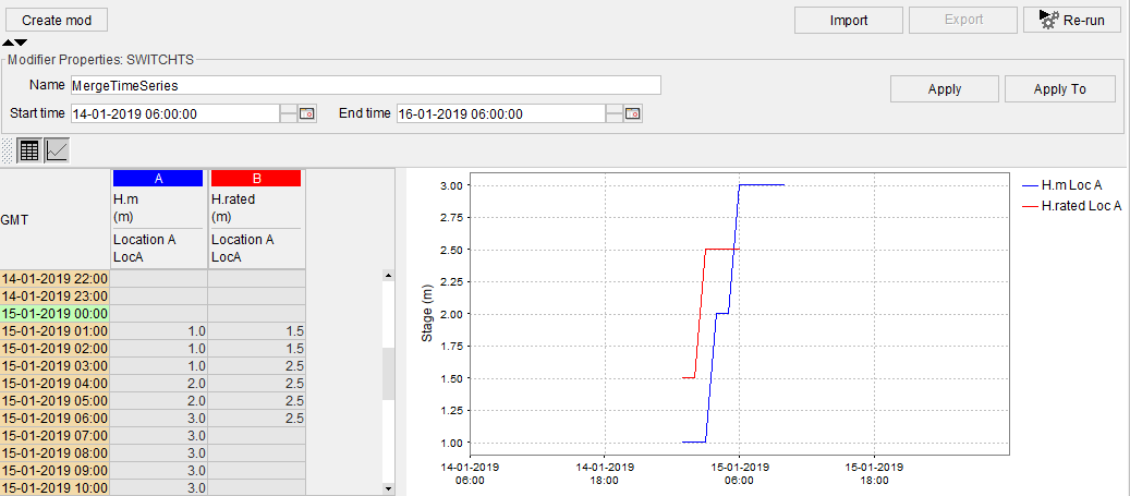
Reverse order modifiers
This modifier can be used to reverse the data hierarchy of the merge simple transformation.
When this modifier is active on the transformation the data hierachy is reversed.
An example of the use of this modifier is the switchts-modifier of the NWS. With this modifier the forecasters temporarily favor one
timeseries above the other because the timeseries which normally is used as the primary timeseries is considered to be less reliable.
Display
Below an example of the display of a reverse order modifier. The display is empty. The forecaster can only set a start- and endtime of the modifier.
If configured it is also to enter a valid time for this modifier.
Schema

Below an example of the display of this modifier. This display is blank, the forecaster can only enter a period in which this modifier is active.
defaultStartTime
The default start time of the modifier. The available options are startrun and time zero.
defaultEndTime
The default end time of the modifier. The available options are time zero and end run.
offsetDefaultEndTime
The offset of the end time compared to the option defined in defaultEndTime.
defaultValidTime
If this option is configured than a valid time can be choosen for this modifier. The valid time always default to time zero.
Configuration example
Below a configuration example.
<mergeSimpleModifiers>
	<reverseOrderModifiers id="switchTs" name="SWITCHTS">
		<defaultStartTime>start run</defaultStartTime>
		<defaultEndTime>time zero</defaultEndTime>
	</reverseOrderModifiers>
</mergeSimpleModifiers>
Rating curve modifiers
Shift rating curve modifiers
Rating curve modifiers are used to modify a rating curve.
The rating curve can be modified by shifting the whole rating curve a constant value or by multiplying it with a factor.
The constant value or the multiplication factor is calculated by the following procedure.
- the forecaster defines a stage/discharge pair,
- from the given stage the discharge is calculated by using the rating curve,
- the difference or factor between the given discharge and the calculated discharge is calculated.
This type of modifier is in use by ncrfc one of the rfc's of the NWS. They use this modifier to temporarily modify the rating curve.
However when new rating curves are available they are imported in their system.
Display
An example of the display of this modifier is shown below. The forecaster can define a stage/discharge pair by defining a pair in the textboxes.
However it is also possible to double click on a point in the graph to define a pair. From the defined stage/discharge pair automatically the constant value
or multiplication factor is derived, which is displayed besides the given stage/discharge pair. The radio button at the top of the display can be used to
switch between the two types of modifier (constant value or percentage).

Schema

defaultStartTime
The default start time of the modifier. The available options are startrun and time zero.
offsetDefaultStartTime
The offset start time compared to the option defined in defaultStartTime. For example when an offset of 1 day is configured
in this option and the defaultStartTime is set to timezero than the default starttime of the modifier will be set to
time zero plus 1 day.
defaultEndTime
The default end time of the modifier. The available options are time zero and end run.
offsetDefaultEndTime
The offset of the end time compared to the option defined in defaultEndTime.
Configuratie voorbeeld
	<ratingCurveModifiers>
		<shiftMultiplyRatingCurveModifier id="qpcshift" name="qpcshift">
			<defaultStartTime>start run</defaultStartTime>
			<defaultEndTime>end run</defaultEndTime>
			<offsetDefaultEndTime unit="day" multiplier="100"/>
		</shiftMultiplyRatingCurveModifier>
	</ratingCurveModifiers>