Introduction

MI-SAFE software and webviewer are developed under the EU funded FP7 project FAST (Foreshore Assessment using Space Technology). The MI-Safe viewer depicts the contribution of coastal vegetation to wave attenuation along global coastlines. MI-Safe is based on global datasets made available via open spatial services and presented in the web-viewer. The data from these global datasets are used to query the results of a modelling exercise with XBeach with a range of conditions worldwide. The results are used to assess requirements for levee design with and without vegetation and give a first estimate of the potential that coastal vegetation has to offer in reducing risk and impact from coastal flood events in areas across the world. 

For background information about the tool, the project and all the partners involved, please visit our website - http://www.fast-space-project.eu/

MI-SAfe data

Elevation

Global SRTM coupled with GEBCO, local DEMS  (why, how and where with links to deliverables/products) (Gerrit/Amrit)

Topography is an important element of the risk of flooding and thus in the MI-SAFE application. Hard rock coasts that rise up from the sea are less vulnerable for flooding than soft sloping sandy coasts. Topography therefore is a very important factor. Several datasets are identified as useful for FAST, these are:

-       SRTM Topography (http://srtm.usgs.gov/)

-       GEBCO Bathymetry (http://www.gebco.net/data_and_products/gridded_bathymetry_data/)

-       ASTER (http://asterweb.jpl.nasa.gov/gdem.asp)

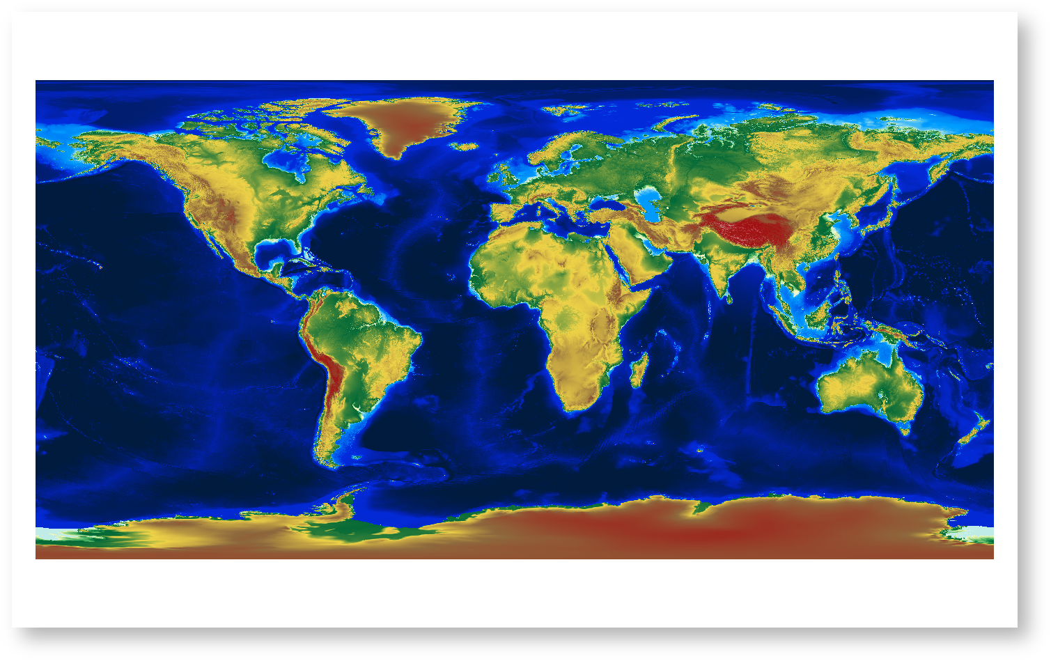
For the global version of the MI-SAFE toolbox a derivative product called SRTM15_plus is used. It offers a continues global coverage of bathymetry and topography. The SRTM15_plus dataset is created by the Scripps Institution of Oceanography (http://topex.ucsd.edu/index.html). This dataset is mainly used for viewing purposes since it is a continues dataset at global level. For use in the MI-SAFE application a more detailed dataset is created using the SRTM3 v4 and GEBCO. The finest resolution of approximately 90 meter is combined where GEBCO is rescaled to 90 meter and interpolated to the SRTM tiles. For performance reasons this is done for tiles along the OSM shoreline of the coast.

Correction with vegetation  (why, how and where with links to deliverables/products) (Arjen Haag)

Method using water levels  (why, how and where with links to deliverables/products) (Ed)

• SRTMplus 15

Waves

Field measurements (why, how and where with links to deliverables/products) (Iris)

Era interim, translated to nearshore depth limited waves  (why, how and where with links to deliverables/products) (Kees)

• era interim wave return periods

Wave data for return periods (T_r) of 1, 10 and 50 years are extracted from the ERA-interim dataset. Waves are generally lower in the tropics (e.g. less than 2 m between -30° to + 30°) than in temperate zones (where H_s>5m between 40°-70°). Below a table with worldwide mean and median values of H_S and T_p from ERA-interim for return periods of 1, 10 and 50 years.

The picture below gives a global view of wave heights for a return period of 1 year.

As the ERA-Interim wave data is based on offshore characteristics, waves are translated to onshore conditions by comparing the waves from ERA-Interim with a depth limited wave. If the depth limited wave height is smaller, this wave height is used for calculations whereas the period is maintained. The wave direction is not taken into account explicitly; the wave direction is assumed to be coast-normal. 

Water levels

Wave attenuation over foreshores is typically most relevant during storm conditions that create a surge (water level set-up) in combination with high tidal levels. For the MI-Safe tool, a water level that has a probability of occurrence of 10%, i.e. once in 10 years, is considered to be the most relevant: This represents a storm that is both frequent enough to appeal to users (a 1/100 or 1/1000 year condition may seem too extreme) and high enough to be a serious threat to coastal regions. The representative water levels or hydraulic boundary conditions are derived from a global D-Flow Flexible Mesh model (Muis et al., 2016) that includes tides, storms and hurricanes. The output of this model is mapped to DIVA segments, so local anomalies can occur for coasts with irregular shapes (bays, estuaries). More extreme or locally tailored conditions can be studied using the more advanced versions of the MI-SAFE tool, which can take into account hydraulic boundary conditions that are specified by users or derived from dedicated modelling.

Vegetation

Field data  (why, how and where with links to deliverables/products) (Iris)

NDVI/LAI  (why, how and where with links to deliverables/products) (Daphne)

Yes/no vegetation map  (why, how and where with links to deliverables/products) (Josh/Ebi)

• global landcover
• global distribution of mangroves

MI-Safe services

MI-Safe provides ....for case study sites. For other foreshore areas in the world MI-Safe reverts to ....

When a user queries a location in the MI-SAFE tool combines data from four parameters to assess the effect of the foreshore on wave attenuation (See Figure Below):

1)      The local (sea)bed level;

2)      The local water level, including tides and storm surge;

3)      The local wave conditions;

4)      The local vegetation type and cover.

To acquire these data for a queried location (point), the tool first determines a transect perpendicular to the nearest coastline. This transect runs 1000 m inland of MSL and 1000 m seaward; the area of interest where most wave attenuation occurs. If relevant vegetation is encountered along this transect, the upper indicator on the left of the screen turns green; if not, red. The properties encountered along this transect are used to find the nearest match in a table that contains wave attenuation results for many thousands of combinations of conditions. The wave attenuation thus obtained is compared to the wave attenuation over a similar but bare transect. If the difference is considerable, i.e. more than the average in this dataset, the lower green indicator turns green too. If the difference is small, the lower indicator displays a red cross.

Surge levels used for the MI-SAFE Expert tool (Jasper, perhaps you can still use some of text below?)

For the Expert version of the MI-Safe tool, locally derived hydraulic boundary conditions have been used wherever available (NL and UK sites) to have the closest resemblance with actual flood defense design conditions.

Wave attenuation over foreshores is typically most relevant during storm conditions that create a surge (water level set-up). For the tool, a water level that occurs once in 10 years was considered to be the most relevant: This represents a storm that both occurs often enough to appeal to the user (a 1/100 or 1/1000 condtion may seem too extreme) and is high enough to be a serious threat to coastal regions. The surge levels are derived from a global surge model (Muis et al., 2016). More extreme or tailored conditions can be studied using the more advanced versions of the MI-SAFE tool.

Wave conditions used for the MI-SAFE Expert tool (Iris/Kees, perhaps you can still use some of text below?)

For waves, a similar reasoning as for surge was followed, leading to the selection of a 1 in 10 year wave height and period. These representative waves are derived from the ERA-interim 40-year reanalysis (ECWMF, 2014).

Schematisation of vegetation types for the MI-SAFE Expert tool (Iris, perhaps you can still use some of text below?).

The MI-SAFE tool needs to function without (yet) having the detailed vegetation properties that are to be determined from EO data. Therefore, vegetation types are derived from existing maps such as the Corine Land Cover (CLC) 2012 and Globcover maps and the characteristics of these vegetation types are based on measurements published in (grey) literature. This document aims to describe how the relevant vegetation types are parameterized in terms of size, density and drag factor for the numerical model that computes the wave attenuation caused by vegetation (XBeach). The basic vegetation

• Salt marshes
• Reed beds
• Riparian willow forests
• Mangroves (only outside Europe)

These vegetation types are not classified as such on the CLC map. A translation from CLC classes to relevant vegetation types has been made, based on the CLC Nomenclature (Corine land cover nomenclature illustrated guide). The details of this reclassification to a ‘simple vegetation map’ are described in the corresponding product specification.

General approach

XBeach requires four parameters to represent the presence of vegetation:

1)      Length or height h (m);

2)      width or diameter d (m);

3)      number of stems per horizontal area n (m^-2);

4)      drag coeffient C_D (-).

Additionally, these can be varied over any number of layers over the vertical to represent plants with a complex morphology (van Rooijen et al. 2016). Worth noticing is that from these parameters, XBeach calculates a ‘vegetation factor’ that is a multiplication of diameter, number and C_d. As a consequence, 200 stems of 1 mm diameter have the same effect as 100 stems of 2 mm diameter.

For deriving representative properties, three principles were followed:

1)      The vegetation factor should be relatively conservative, so as not to give an overly optimistic estimate of wave attenuation. Thus, plant dimensions are chosen with winter conditions and relatively small individuals in mind. The choice of the drag coefficient beforehand is troublesome, because this not only depends on the plant properties but also on the hydrodynamic conditions. Therefore, a relatively conservative estimate is made with large waves (that give large Reynolds/Keulegan-Carpenter numbers that are associated with low drag coefficient values) and the flexibility of the vegetation in mind. This will be refined once more reliable drag coefficient estimators are available, e.g. based on observations from the FAST field sites.

2)      The vegetation factor should be representative for all occurrences of a particular type across Europe, not for a specific site.

3)      The vegetation factor should be large enough and differ enough between vegetation types to meaningfully differentiate the effects of different vegetation covers from each other.

Note that these basic assumptions are used if only global information is available in the Educational version of the tool at present. In the Expert version, the local EO data will be used to derive vegetation properties.

Intertidal vegetation (salt marshes)

Intertidal vegetation is derived from the CLC class Salt marshes (421): areas submerged by high tides where vegetation dominates. The cover of such marshes can vary considerably between locations and throughout the year. For example, Spartina spp  stands can well be 70 cm high during summer, whereas Salicornia spp.  can be nearly absent in winter. The properties as observed by Möller et al (2014) were selected as representative (Table 1), because they are for a mixed marsh typical for North-Western Europe and because they were measured with wave attenuation studies in mind rather than just observing biomass. Moreover, the drag coefficient of that particular vegetation cover has been derived from large-scale flume experiments under (near) real world wave conditions.

Inland marsh (reed beds)

Reed beds are of interest for inland locations such as lakes that are often fringed by reed beds, and for the Romanian study sites of FAST where large reeds grow in coastal lagoons. The CLC map does not account for reed beds as such, but are based on class 411 Inland marsh. As a result, the MI-SAFE tool will apply reed bed properties to every inland marsh, also the ones predominantly made up of lower shrubs, and might overestimate the wave attenuation capacity of such marshes.

For the moment, the properties of the reed beds at the Romanian sites (Table 1) have been used because these are readily available and because they represent the situation at the study site, which enables a comparison with local observations of wave attenuation. It should be noted that these are possibly taller reeds than usually found along lake banks.

Riparian willow forests (broadleaved forest)

All areas classified by CLC as ‘broad leaved deciduous forests’ (class 311) are considered to be willow forests if they are located in Europe, where no mangroves occur. The CLC class also contains many forests far from any large water body, but these are not relevant as they will not be queried by users of the MI-Safe tool. Forests hardly occur directly adjacent to the coastline, and if they do they are usually coniferous so they will not lead to a false positive identification as willow forest. As a consequence, riparian forests are the most likely forests to be identified in this class.

The composition, and consequently tree size, of riparian forests differs considerably among floodplains but willows are very common in European floodplains. The age and size of willows depends strongly on the management of floodplains: in natural rivers they are older and taller than along strictly managed rivers, where they can be cut regularly to prevent flooding as a result of the additional hydraulic resistance they cause. Such managed areas are more likely to be of interest, and the MI-Safe tool should not overestimate the wave attenuating effect. Therefore, the willow dimensions are chosen to be representative of relatively young, regularly trimmed trees. Data are available from sites in the Netherlands: commonly found regularly cut pollard willows (‘knotwilgen’) of several years old and young willows (less than 1 year old) of a field especially planted for wave attenuation in front of a levee near Fort Steurgat, Werkendam. 

The wave model: XBeach (Jasper, perhaps you can still use some of this text below?)

In order to quantify wave attenuation by vegetation for a given salt marsh coastline (see example in Figure XX), the numerical modeling software XBeach (van Rooien et al. 2016) was used. Xbeach is a depth-averaged, two-dimensional process-based model that solves the time dependent short wave action balance for the entire wave group. XBeach has three processes that occur on a short wave scale that are able to be incorporated in simulations: dissipation due to wave breaking, dissipation due to bottom friction, and dissipation due to vegetation. 

The viewer (Gerrit, Amrit, Arjen, Ed, perhaps you can still use some of this text below?)

The viewer is build up of 3 main parts; the canvas where the maps are shown, the data part where a selection of layers can be toggled on or of and the results. The results part enables users to draw a profile of the coast. Via OGC services (a WPS in this case) data is extracted over the profile. This data is then classified for certain characteristics, such as elevation, water levels, wave charateristics and vegetation presence and type. This data is then used to query the table of model results. The result is shown  indicating whether or not vegetation is existent and or contributes to wave attenuation. 

The case study sites

UK (Iris)

Could you include some background information on the case study areas, i.e. a short description of the vegetation, natural wave climate, extreme conditions and any other relevant information? A starting point would be the case study descriptions in the DoW, but they do need to be updated.

The Netherlands (Daphne)

Could you include some background information on the case study areas, i.e. a short description of the vegetation, natural wave climate, extreme conditions and any other relevant information? A starting point would be the case study descriptions in the DoW, but they do need to be updated.

Spain (Gloria)

Could you include some background information on the case study areas, i.e. a short description of the vegetation, natural wave climate, extreme conditions and any other relevant information? A starting point would be the case study descriptions in the DoW, but they do need to be updated.

Romania (Albert)

Could you include some background information on the case study areas, i.e. a short description of the vegetation, natural wave climate, extreme conditions and any other relevant information? A starting point would be the case study descriptions in the DoW, but they do need to be updated.