What is the IFD?
The IFD is short for Interactive Forecast Displays.
The IFD is a set of displays which enable the forecaster to create a forecast manually in comparison to a batch run which creates a forecast in a background process triggered either by a schedule or manually.
When a forecaster creates a forecast in the IFD, the forecast created in the background process is usually used as the starting point for the forecaster.
The forecaster validates the results from the server run and adjusts the forecast by using modifiers were needed.
When the forecaster is satisfied with the adjusted forecast the forecast is finalized and published to other forecasters.
Usually when creating a forecast by using the IFD, FEWS runs in a mode where all the windows are dockable.
This is an important aspect of the IFD because this feature enables the forecaster to keep an overview of the system.
Contents
Which displays are used in the IFD?
The IFD consists of several panels.
Each of these panels has a specific role in the process of creating a forecast with the IFD.
In this chapter the functionality of each panel in the IFD will be explained.
In the next chapter will be explained with a use case how a forecast can be created with the
IFD by using the combined functionality of the separate panels.
Forecast panel

The forecast panel plays a central role in creating a forecast in the IFD.
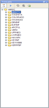
The forecast panel shows a tree with all the forecast points for a region and the grouping of these forecast points.
Each node in the tree can be linked to a workflow. For example node EAGLE NEST DAM has its own workflow.
Each node also shows the current status of the last run of the workflow to which the node refers.
Workflows of parent nodes are always run on the server. By default leaf nodes are locally run, however it is also possible that these workflows are run on the server.
This can be done by setting the optional tag localRun to false for a node.
The leaf nodes are indicated by the small black balls in the display, parent nodes (node containing other parent nodes or leafs) are indicated as a folder in the forecast display.
When a leaf node is selected the ifd will automaticly run the workflow of that node.
This behaviour can however be disabled in the configuration by setting the enableAutoRun-tag to false in the topolog.xml.

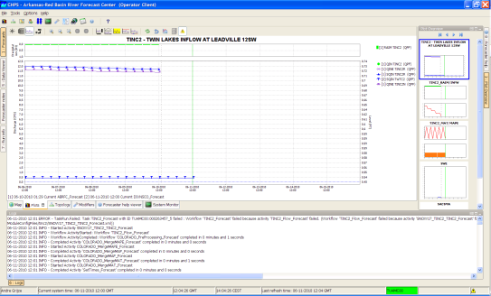
If the node shows a green checkbox (as is seen in the image above at the node DIVERSIONS-CO) item it means that the workflow has run successfully.
A red exclamation (as is seen in the image above at the LEADVILLE node) mark indicates that the workflow is failed.
A yellow ball indicates that the workflow was successful in a prior run, but the results have since been invalidated by some upstream change.
For example, when the forecaster has created a modifier but did not rerun the workflow yet.
Or when an upstream node was run later than one off its downstream nodes then the results of the downstream nodes are set to invalid.
When a folder is shown for a parent node (as is seen for the COLORADO node in the image below) or a black ball for a leaf node (as is seen in the MALTA 5SE node) then the workflow has not run yet for the current time zero.
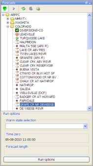
A green arrow (as is seen in the node TURQUOISE LAKE) indicates that the workflow is currently running (locally or at server).
An hour glass (see node HALFMOON above) indicates the workflow is scheduled to run.
Go to next segmentAdjust T0
Run on ServerForecast/View-button

Re-Run button
At the top of the forecast panel several buttons are shown.
The first button is a Forecast/View toggle button (Put image of the button here) which can be used to switch from View mode to Forecast mode.
In the Forecast mode the forecaster can create modifiers and when a leaf node is selected the workflow is run automatically . In View mode the forecaster can view the results of other forecasts.
However, it is not allowed to create modifiers and workflows will not be run automatically when a node is selected. A workflow can be forced to run by pressing the Re-Run button.
The second button is the Go to Next Segment-button (image of button here). By pressing this button automatically the next leaf-node in the forecast panel will be selected.
The third button is the Re-Run-button (need button image). This button is only enabled when a node is selected which has a workflow which runs locally.
The fourth button is the 'Run on Server'-button (need button image here). This button is only enabled when a node is selected with a workflow which should run on the server.
The last button is the Adjust T0 (need image of button) button which allows the forecaster to adjust the current system time to the nearest cardinal time step prior to the current time.

At the bottom of the forecast panel there is a Run options section. In this section the forecaster can set the properties of the run. The warm state can be selected and the current Time zero is also displayed. More advanced options are available with the button Run options.
Modifiers panel
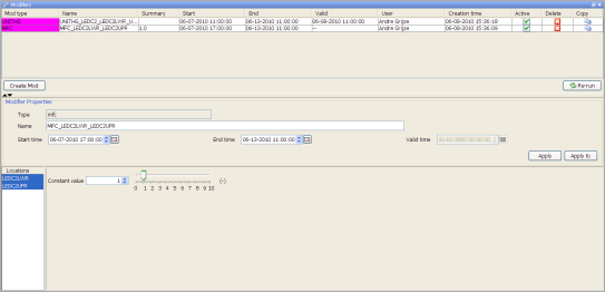
The modifiers panel is an important display in the IFD.
It shows the modifiers which are created for a certain node. Modifiers can be created, modified or deleted in this panel.
The upper part of the display gives an overview of the modifiers created for the currently selected node in the forecaster panel.
It lists the Start Date, the End Date, the Valid Date and the Creation time of the mod.
It also allows the user to make mods active and inactive with the checkbox in the column Active.
A mod can be deleted by pressing the red cross icon and a copy can be made pressing the copy-icon.

With the create mod-button the forecaster can create new modifiers. When the button is pressed a dropdown-list with the available modifier types for the currently selected node is shown.
The modifiers which are shown are depended on the models, transformations and module parameterfiles available in the workflow of the selected node and the plots which are associated with the node.
In the modifierTypes.xml is defined which modifiers are available for the forecaster. The combination of the configuration of the modifierTypes.xml and the workflow and the time series in the plots
When a modifier type is selected, the details of the new modifier is shown is in the lower part of the display. In some cases it is also necessary to specify to which models the modifier should be applied.
For example when the forecaster selects the modifier type MFC and there are two SNOW17-models available in the segment, the forecaster should also specify to which models the modifier should be applied.
When the modifier can be applied to more than one model in a basin a 'location'-panel shows up at the left part of the details display. In this panel the forecaster can select to which locations the modifier should be applied.
The Re-run button runs the workflow from the selected node and the workflows from the upstream nodes.
The lower part of the display shows the details of the selected modifier or when the forecaster is creating a new modifier the details of the new modifier.
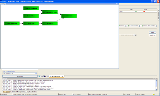
Topology panel
The topology panel shows the topology of the selected node. When a leaf node is selected the topology of the parent node is shown. When a parent node is selected the topology of its children is shown.
The colors of the boxes in the topology change when a threshold is passed. The color of the box and the thresholds which are monitored can be configured.

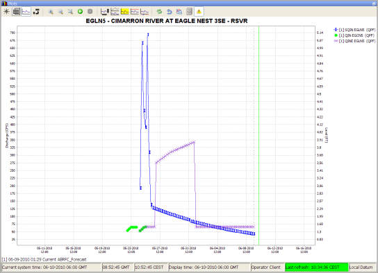
Plot
The plot display is used to show scalar time series. Each node has its own set of predefined displays configured. When a node is selected the plots display automatically updates the plots which are already displayed to show data for the new node. The first plot configured for the selected node is automatically shown in this display.
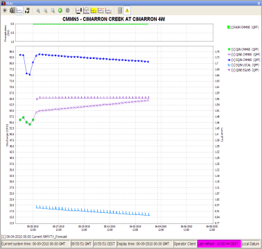
When the IFD is started, there is always at least one plot display available. This plot is called the primary plot display. The primary plot doesn't have lock icon at the left of the toolbar. When a new plot display is started this plot will have a lock icon at the left on the toolbar. When a new plot displayed is started, by default the plot will be locked.

When a plot is locked, the display is locked to that set of time series. When the forecaster moves from basin to basin, the plot will continue to display the original timeseries. The plot is not updated. However, as new data is brought in, the plot is updated with new data.
When the toggle-button is switched off (icon changes to unlock) the plot window is updated automatically when a new node is selected.
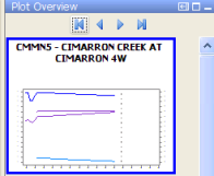
Plot overview
The plot overview is a panel which shows a thumbnail of each plot which is configured for the selected node. This panel gives an overview of the selected node. When a plot is selected the primary plot is automatically updated, also other plots display which are not locked (see previous chapter) are updated.

At the top of the panel there are four buttons. The first button selects the first plot, the second button selects the previous plot, the third button selects the next plot and the last button selects the last plot.
Forecaster help
The forecaster help panel shows user provided documentation which is available for a node. Currently the following formats are supported: textfiles, images and pdf-files. Users can place documents in a directory within a predefined directory. This directory can be configured in the global.properties by defining the INFORMATION_PANEL_FOLDER property.
Within this directory each node has its own directory. The directory should have the same name as the node id. Within that directory that documentation for that node can be placed.
Below an example of the tool window forecaster help. In this example the forecaster has two documents available for information.
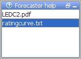
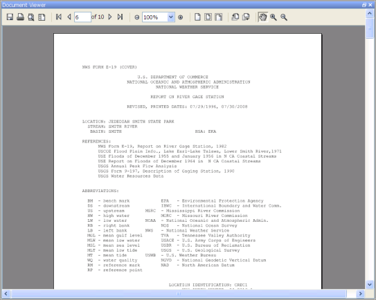
When one of the files is selected in this panel the content of the selected file is shown in the document viewer. The document viewer is a dockable window in the centre of FEWS.
The content of the forecast help dialog is depended of which node is selected in the forecaster panel. When a new node is selected the content of the forecaster help dialog is automatically updated.
Run info
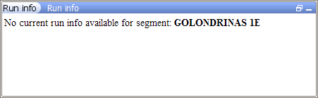
The run info panel shows detail information of the latest run of the workflow of the selected node. If the workflow of the node has not run yet for the current T0 then the panel will show that there is no current run info available
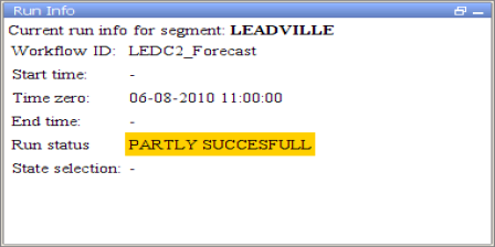
When the workflow has run. The status can either be succesfull, failed or partly successful. Only when the workflow was succesfull than the icon of that node will be set to green. The run status will be shown green in the run info box.

When the run is partly successful the icon of that node will be set to the red exclamation mark, the run status box in the run info panel will be set to yellow. When the run is failed the icon of the node will be set to the red exclamation mark, the run status box will be set to red.
Forecaster notes
The forecaster notes panel shows the notes other forecaster have created regarding their previous forecasts for the forecast point. Forecasters can also created their own note and publish them.

Modifiers
Introduction
A forecaster can modify a forecast with so-called Modifiers. Within FEWS there are two types of modifiers: time series modifiers and parameter modifiers. Parameter modifiers can modify a parameter of a model or of a transformation.
Time series modifiers modify a time series. The original time series is stored in the database. However as soon as this time series is retrieved from the database the modifier will be applied to it. But it is important to note that the original time series is always available in the database.
Time series modifiers
Single value modifiers
A single value modifier is a modifier which modifies only one value at one time step in a time series. The display which is used for single value modifiers is shown below.

The user can enter a value in the text box by entering a value and by clicking on the spiner box next to it. The value can also be adjusted by the slider bar on the right side of FEWS.
In the example above we see the display of the single value modifier WECHNG. The WECHNG mod sets the value of the snow water equivalent in a specific snow model at one point in time. Below the configuration of this modifier is shown.
<singleValueModifier id="wechng" name="WECHNG">
<timeSeries>
<parameterId>WECHNG</parameterId>
</timeSeries>
<softLimits>
<maximumValue>5</maximumValue>
<minimumValue>0</minimumValue>
</softLimits>
<hardLimits>
<minimumValue>0</minimumValue>
</hardLimits>
<defaultTime>start run</defaultTime>
<defaultValue>0</defaultValue>
</singleValueModifier>
First the id and name of the modifier is declared. The timeSeries-part identifies that this modifier can be applied to any time series which have the parameter WECHNG. The modifiers has some soft limits. These limits are used to limit the slider bar in the display. In this case the slider bar will start at 0 and end at 5. But these soft limits can be overruled by manually typing a value lower than zero or higher than 5. The hardLimits identify the upper and lower limit of the mod and they can not be overruled. This means that for this mod only the maximum value of the soft limit of 5 can be overruled. A single value modifier is only applied at one time step. By default this is set to the start of the run in this modifier. The default value is set to 0.
Constant value modifiers
Constant value modifiers are very similar to single value modifiers. But instead of modifying a single value at a particular point in time, they modify a time series over a period of time with a fixed value. Below the display of a constant value modifier is shown. Which is very similar to the display of single value modifier. Note however that this modifier has a start and an end time.

Below an example configuration of a constant value modifer is shown.
<constantValueModifier id="mfc" name="MFC">
<timeSeries>
<parameterId>MFC</parameterId>
</timeSeries>
<softLimits>
<maximumValue>10</maximumValue>
<minimumValue>0</minimumValue>
</softLimits>
<defaultStartTime>start run</defaultStartTime>
<defaultEndTime>end run</defaultEndTime>
<defaultValue>1</defaultValue>
</constantValueModifier>
The only difference in the configuration of a constant value modifier and a single value modifier is that a default start- and endtime should be configured instead of default time.
Enumaration modifiers
Below an example of the display for an enumeration modifier.

In this type of modifier the forecaster can select several options from a dropdownlist. Each option is translated to a certain value in the time series.
Below is an example of the configuration of an enumeration modifier.
<enumerationModifier id="rainsnow" name="RAINSNOW">
<timeSeries>
<parameterId>RAINSNOW</parameterId>
</timeSeries>
<descriptionEnumeration>choose precipitation:</descriptionEnumeration>
<enumeration>
<item text="rain" value="1"/>
<item text="snow" value="2"/>
</enumeration>
<defaultStartTime>start run</defaultStartTime>
<defaultEndTime>end run</defaultEndTime>
</enumerationModifier>
This modifier is applied to every time series which has parameter id RAINSNOW because a filter is defined with only the parameterId RAINSNOW.
The text of the label in front of the dropdownlist is configurable. The items in the dropdownlist are also configurable. For this modifier the forecaster can choose between options rain and snow. If snow is selected a value of 2 in set into the time series for the selected period. If rain is selected a value of 1 is written into the time series. The numbers are treated as flags by the model to which the time series is passed.
Time series modifier
The time series modifier is a modifier which directly edits a certain time series. In the example below the display for the RunOff Change (ROCHNG) modifier which is configured to change the model produced runoff. The forecaster can edit this time series by making changes in table or in the graph. The changes in the graph are made by clicking in the graph. When the user clicks from left to right then the values between the points are interpolated. When the user clicks from right to left only the newly added or changed points are adjusted but no interpolation will be done between the last two points. When more than one time series is shown in the display it is possible to make a selection of which time series should edited when making changes by clicking in the graph. The time series which should be changed can be selected by clicking on the legend of that example time series in the graph.

Below is an example of how a time series modifier should be configured.
<timeSeriesModifier id="rochng" name="ROCHNG">
<timeSeries>
<moduleInstanceSetId>SACSMA_Forecast</moduleInstanceSetId>
<valueType>scalar</valueType>
<parameterId>INFW</parameterId>
<locationSetId>Gages_Catchments</locationSetId>
<timeSeriesType>simulated forecasting</timeSeriesType>
<timeStep unit="hour" multiplier="6"/>
<ensembleId>QPF</ensembleId>
</timeSeries>
<defaultStartTime>start run</defaultStartTime>
<defaultEndTime>end run</defaultEndTime>
<resolveInWorkflow>true</resolveInWorkflow>
<resolveInPlots>false</resolveInPlots>
</timeSeriesModifier>
This modifier can be applied to the time series identified in tag timeseries. The modifier will have a start time equal to the start of the run and will end at the end of the run. The option resolveInWorkflow is set to true and the option resolveInPlots is set to false. This means that the IFD will search for time series which might be modified in the workflow of the selected node but it will not search in the time series which are displayed in the plots for this node.
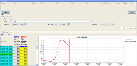
Mark unreliable modifier
This modifier sets all the values in a time series to unreliable over a period so the data will not be used in the models, but the original values will be displayed.
The forecaster can only edit the start and end dates of the period in which the time series will be set to invalid. In the Modifiers Display table the unreliable values in the modified time series are marked yellow.
Below an configuration example of this type of modifier
<markUnreliableModifier id="ignorets" name="IGNORETS">
<timeSeries>
<moduleInstanceSetId>RESSNGL_Forecast</moduleInstanceSetId>
<valueType>scalar</valueType>
<parameterId>PELV</parameterId>
<locationSetId>Reservoirs</locationSetId>
<timeSeriesType>simulated forecasting</timeSeriesType>
<timeStep unit="hour" multiplier="1"/>
</timeSeries>
<defaultStartTime>start run</defaultStartTime>
<defaultEndTime>end run</defaultEndTime>
</markUnreliableModifier>
In the tag time series can be specified to which time series this modifier can be applied. In the tag defaultStartTime the default start of the modifier can be specified. The configuration can choose start run or time zero. The tag defaultEndTime can be used to specify the default end time of the modifier. The configuration can choose time zero or end run.
Compound modifier
The compound modifier can be used to modify a set of time series with slider bars. Each slider shows a reference value in blue and the modified value. Initially the modified value is equal to the reference value. For each slider there is a time series configured which stores the modified value and a time series configured which holds the reference value. This type of modifier is typically used as a state modifier of models. The reference values show the current state of the model. The modified values in the boxes show the modified state values. The maximum value of the slider bar is derived from a parameter in the linked module parameter file.

Below an example of the configuration of a compound modifier. In this example a part of the sacco configuration is not shown but only the configuration of one of the five sliders is shown.
For each slider the time series which holds the reference values should be configured, and the time series which should contain the modified value should be configured. Each slider also has maximum value. This maximum is retrieved from the module parameter file of the model. The tag maximumAllowedValueParameterId identifies which parameter should be used to identify the maximum.
<compoundModifier id="sacco" name="SACCO">
<slider>
<currentTimeSeries>
<moduleInstanceSetId>SACSMA_Forecast</moduleInstanceSetId>
<valueType>scalar</valueType>
<parameterId>UZTWC</parameterId>
<locationSetId>Gages_Catchments</locationSetId>
<timeSeriesType>simulated forecasting</timeSeriesType>
<timeStep unit="hour" multiplier="6"/>
</currentTimeSeries>
<modifiedTimeSeries>
<moduleInstanceId>ExportMODS</moduleInstanceId>
<valueType>scalar</valueType>
<parameterId>UZTWC</parameterId>
<locationSetId>Gages_Catchments</locationSetId>
<timeSeriesType>external historical</timeSeriesType>
<timeStep unit="nonequidistant"/>
</modifiedTimeSeries>
<maximumAllowedValueParameterId>UZTWM</maximumAllowedValueParameterId>
</slider>
<defaultTime>start run</defaultTime>
</compoundModifier>
The default time of the model can also be configured. The configurator can choose between start run or time zero.
Missing value modifier
The missing value modifier can be used to set the values in a time series to missing over a period of time.

Like the Mark Unreliable Modifier, for the Missing Value modifier, the forecaster can only edit the start date and the end date of period in which the values of the time series should be set to missing. In the table and the graph of the Modifiers Display the values of the modified time series are not shown when they have been set to missing.
Below an example of the configuration of a missing value modifier.
<missingValueModifier id="setmsng" name="setmsng">
<defaultStartTime>start run</defaultStartTime>
<defaultEndTime>end run</defaultEndTime>
<resolveInWorkflow>false</resolveInWorkflow>
<resolveInPlots>true</resolveInPlots>
</missingValueModifier>
The tag resolveInWorkflow is set to false and the resolveInPlots tag is set to true which means that the modifier can be applied to all time series in the plots of the node, but will not be applied to the time series identified in the workflow of the node. In this example there are no time series defined to which this modifier should be applied. This means it can applied to all time series which are defined in the plots of a node.
Switch option modifier
This modifier allows the forecaster to generate several linked time series. This modifier is currently used to set regulation options for a basin. For each regulation option a time series should be identified. There are two types of time series which can be configured, time series in which the forecaster can enter any value and time series which can only contain a 1 when the option is switched on.
Below an example of the display of a switch option modifier.

For each data at a model time step one of the options can be selected by the radio-button-field. In the value field the forecaster can enter a value or if the option is only a switch on option, the value field is blocked. The add-icon automatically adds a new entry to the table. By default the new entry will have the data of the current row plus one model time step. The delete-icon deletes all the selected rows. The entries are allways in sequence.
Below an example of a switch option modifier. For each regulation option available in the display a time series should be defined. The parameterid of the configured time series will be used as the name of the regulation option in the column regulation.
<switchOptionModifier id="ssarreg" name="ssarreg">
<timeValueTimeSeries>
<moduleInstanceId>ExportMODS</moduleInstanceId>
<valueType>scalar</valueType>
<parameterId>SETH</parameterId>
<qualifierId>US</qualifierId>
<locationSetId>ImportIHFSDB</locationSetId>
<timeSeriesType>external forecasting</timeSeriesType>
<timeStep unit="nonequidistant"/>
<ensembleId>main</ensembleId>
</timeValueTimeSeries>
<timeValueTimeSeries>
<moduleInstanceId>ExportMODS</moduleInstanceId>
<valueType>scalar</valueType>
<parameterId>SETQ</parameterId>
<qualifierId>US</qualifierId>
<locationSetId>ImportIHFSDB</locationSetId>
<timeSeriesType>external forecasting</timeSeriesType>
<timeStep unit="nonequidistant"/>
<ensembleId>main</ensembleId>
</timeValueTimeSeries>
<timeValueTimeSeries>
<moduleInstanceId>ExportMODS</moduleInstanceId>
<valueType>scalar</valueType>
<parameterId>SETS</parameterId>
<qualifierId>US</qualifierId>
<locationSetId>ImportIHFSDB</locationSetId>
<timeSeriesType>external forecasting</timeSeriesType>
<timeStep unit="nonequidistant"/>
<ensembleId>main</ensembleId>
</timeValueTimeSeries>
<timeValueTimeSeries>
<moduleInstanceId>ExportMODS</moduleInstanceId>
<valueType>scalar</valueType>
<parameterId>SETDH</parameterId>
<qualifierId>US</qualifierId>
<locationSetId>ImportIHFSDB</locationSetId>
<timeSeriesType>external forecasting</timeSeriesType>
<timeStep unit="nonequidistant"/>
<ensembleId>main</ensembleId>
</timeValueTimeSeries>
<timeValueTimeSeries>
<moduleInstanceId>ExportMODS</moduleInstanceId>
<valueType>scalar</valueType>
<parameterId>SETDQ</parameterId>
<qualifierId>US</qualifierId>
<locationSetId>ImportIHFSDB</locationSetId>
<timeSeriesType>external forecasting</timeSeriesType>
<timeStep unit="nonequidistant"/>
<ensembleId>main</ensembleId>
</timeValueTimeSeries>
<booleanTimeSeries>
<moduleInstanceId>ExportMODS</moduleInstanceId>
<valueType>scalar</valueType>
<parameterId>FREEFLOW</parameterId>
<qualifierId>US</qualifierId>
<locationSetId>ImportIHFSDB</locationSetId>
<timeSeriesType>external forecasting</timeSeriesType>
<timeStep unit="nonequidistant"/>
<ensembleId>main</ensembleId>
</booleanTimeSeries>
<timeValueTimeSeries>
<moduleInstanceId>ExportMODS</moduleInstanceId>
<valueType>scalar</valueType>
<parameterId>SETDS</parameterId>
<qualifierId>US</qualifierId>
<locationSetId>ImportIHFSDB</locationSetId>
<timeSeriesType>external forecasting</timeSeriesType>
<timeStep unit="nonequidistant"/>
<ensembleId>main</ensembleId>
</timeValueTimeSeries>
<startTime>start run</startTime>
<effectiveDate></effectiveDate>
</switchOptionModifier>
Module parameter modifiers
Blending steps modifier
One of the parameters of the adjustQ-transformation is the blending steps. This parameter determines in how many steps the blend from the observed time series to the simulated time series is done. Below is an example of a blending steps modifier. The forecaster can enter the value in the text box and/or change it with the up and down arrows next to the text box.

Below an example of the configuration an adjustQModifier. The only thing the configurator has to configure is the id of the modifier and its name.
<adjustQModifiers>
<blendingStepsModifier id="chgblend" name="chgblend"></blendingStepsModifier>
</adjustQModifiers>
Sample years modifier
The transformation sample historic creates ensembles based on historic time series. This modifier enables the forecaster to change the start year and the end year of the historic time series to sample.
Below an example of the display of this modifier.

The forecaster can modifiy the default sample years by changing the start year and end year in the display.
Below an example of the configuration of this modifier.
<sampleHistoricalModifiers>
<sampleYearsModifier id="historicwateryears" name="historicwateryears"></sampleYearsModifier>
</sampleHistoricalModifiers>
Module parameter modifier
The module parameter is a generic modifier which can be used to edit any type of module parameter file. Below an example of the display of a module parameter modifier. In this example only one parameter can be modified.

Below an example of the configuration of a module parameter modifier. With the tag filter can be identified which module parameter files can be modified. In the example below every module parameter file with the tag CONSTANT_BASE_FLOW can be modified. The filter is also used to filter which part of the module parameter file can be modified. In the example below only the module parameters with id CONSTANT_BASE_FLOW are shown in the modifiers display and are editable.
<moduleParameterModifier id="baseflow" name="BASEFLOW">
<filter>
<moduleParameterId>CONSTANT_BASE_FLOW</moduleParameterId>
</filter>
<defaultValidTime/>
</moduleParameterModifier>
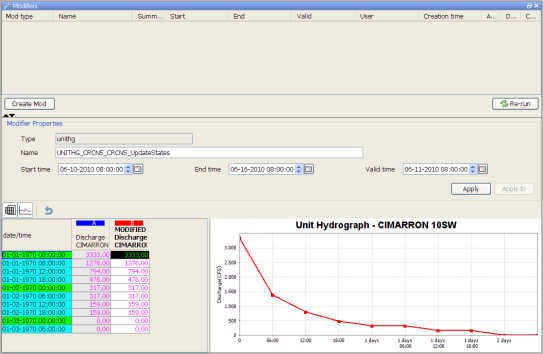
Change ordinates modifier
This modifier can be used to change the ordinates of the module parameter file of the unit Hydrograph-model. Below an example of the display of this modifier. The ordinates can be changed in the table or in the graph. When the user presses the apply button the ordinates are adjusted by using a volume-correction. The volume correcton will ensure that the volume without the modifier applied is the same as the volume of unit hydrograph after the modifier is applied.
Below an example of the configuration of this modifier.
<unitHydrographModifiers>
<changeOrdinatesModifier id="unithg" name="UNITHG">
<defaultStartTime>start run</defaultStartTime>
<defaultEndTime>end run</defaultEndTime>
<defaultValidTime/>
</changeOrdinatesModifier>
</unitHydrographModifiers>
Reverse order modifiers
This modifier can be used to reverse the data hierarchy of the merge simple transformation. When this modifier is active on the transformation the data hierachy is reversed. Below an example of the display of this modifier. This display is blank, the forecaster can only enter a period in which this modifier is active.

Below a configuration example.
<mergeSimpleModifiers>
<reverseOrderModifiers id="switchTs" name="SWITCHTS">
<defaultStartTime>start run</defaultStartTime>
<defaultEndTime>time zero</defaultEndTime>
</reverseOrderModifiers>
</mergeSimpleModifiers>
How to create a forecast with the IFD
Steps in creating a forecast
Below is a list of all possible steps in creating a forecast with the IFD. Please note that not all of the listed steps are obligated. For each step will be explained how this step can be carried out using the IFD in FEWS.
- Start FEWS
- Selecting the forecast panel
- Reviewing the topology
- Review the list of available state date/times
- Adjust state and/or forecast length
- Starting the forecast process and selecting the workflow for which the forecast should be made
- Reviewing workflow status
- Reviewing graphs (graph display listens to segment selection)
- Reviewing graphs (graph display is independed from segment selection)
- Continue with the forecast process downstream
- Ending the forecast process
Starting FEWS
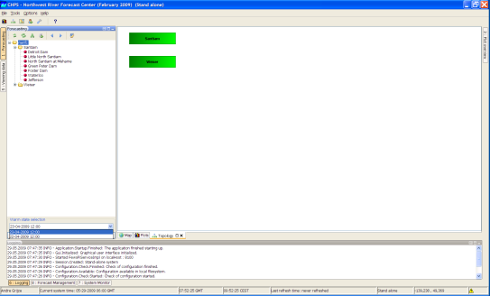
After starting FEWS, the map-display will be displayed in the centre and the Forecast Panel-tab at the left will be selected. This the default layout. The layout after starting FEWS is however configurable by creating and saving a custom layout by using the option in the File menu at the top left of the display.

First the IFD will try to synchronize the local datastore with the central database. Until that process is finished it is not possible to create a forecast with the IFD. To indicate that the IFD is doing its initial synchronization after startup the forecast-button shows a hour glass icon. While the Operator Client if synchronizing, it is possible to view scalar and spatial data.
When the initial synchronization is finished. The following message is shown.

Selecting the forecast panel
The whole process of creating of forecast by using the IFD is managed by the forecast dialog, therefore the first step is selecting the Forecast tab at the left of the display. The Forecast tab will give an list, in computational order of the basins of the region.

Review the list of available state date/times
The forecast panel also shows at the bottom the currently selected (default) warm state. By clicking on the drop-down box all the available warm states are shown. If the forecaster needs to use a different warm state than the default, a new warm state date may be selected from drop down menu titled Warm State Selection. If the default warm state is not correct another warm state can be selected from the drop-down box.
Adjust state and/or forecast length
By pressing the Run Options button at the bottom of the forecast dialog the user will have access to alternative ways of selecting states. After pressing the advanced button a dialog will be shown in which the user can select the state, forecast length and a what-if scenario.

After selecting the OK-button the selected state or forecast length will be applied and used in the runs.
Starting the forecast process
To start the interactive forecast process, the user should select a leaf node. If the IFD is in forecast mode (which it is by default) the workflow of the selected node will also be automatically run. Models can be run by selecting a node, or pressing the rerun button.
In view mode the forecaster can view data but it is not possible to create a forecast.
Reviewing run status workflow
When a run is finished the segment-dialog will show the status of the run. If a run is in progress a refresh-icon will be shown. A green box will indicate a successful run. A red exclamation mark will indicate that run workflow has failed. A yellow dot will indicate the workflow has run succesfully but that the results are invalid. For example when an upstream segment has run later than the workflow for a downstream segment the results of the downstream segment workflow are invalid.
The icons displayed on the leaf node (for individual basins) indicate the status of local runs. If the icon is blank then the server run is the most recent run. Icons on the parent nodes indicate the status of server runs.

Review graphs (graph display listens to segment selection)
When a basin run has finished the results of the run should be reviewed. By selecting the plot overview at the right a list of thumbnails will be displayed. For each graph available for the current node a thumbnail will be shown. To display a graph, the forecaster selects a thumbnail and then this graph is displayed in the main plot window. The plot display will show the selected graph. Navigation between the graphs can be done by selecting a graph by clicking on a thumbnail with the mouse or by pressing alt+g (go to next graph) or by pressing shift+alt+g(go to previous graph). When the Thumbnail Panel is selected it is also possible to navigate by using the arrow keys up and down on that panel. When a new node is selected in the Forecast Tab the list of thumbnails is automatically updated to show the graphs available for the newly selected node.
The Plot Overview panel can be undocked. When the display is expanded the plots are automatically resized.

Creating a mod in the time series display
Mods can be created in the mods display or directly in the plot display. To modify a time series directly in a plot, a time series has to be selected. This can be done by selecting a time series in the legend of the plot. To indicate that a time series is selected the legend and the time series will be plotted bold.

Creating a mod in the mods display
The modifier display can be started by clicking on the wrench-icon at the toolbar or by using the shortcut ctrl+m. The modifier display will show all the mods which are applied in the currently selected segment. By clicking on the create mod-button a new mod can be created. After pressing the create mod-button a list of available mods will be shown. When the mod is created it can be applied by pressing the apply-button. With the run-buttons (rerun, rerun to selected and rerun all to selected) it is possible to rerun the workflows. Pressing the run-buttons will also automatically apply the mod.
Continue with the forecast process downstream
After reviewing the graphs and if needed applying mods the forecaster can proceed to the next segment. Going to the next segment can be done easily by pressing alt+s (go to next segment) or by pressing the next segment-button in the forecast panel or by selecting the next node. After selecting the segment the workflow will be run automatically and after finishing the run the status of the run will be shown by color of the dot of the segment.
Ending the forecast process
When the forecaster thinks that the current forecast is sufficient. The forecast can select the parent node of the leaf nodes and press the 'run on server'-button. When this button is pressed, first all the new modifiers and changes to the existing modifiers of the child nodes of the selected node will be uploaded to the server. When the upload is successful the workflow will be run at the server. The locally created runs will be deleted when the server run was successful and the results are downloaded successfully back to the Operator Client.
Dockable windows
Docking and undocking main displays
All windows in the centre section of FEWS can be undocked. This can easily be done by clicking on the square-box icon beside the x-icon at the tab of each display. Undocking the windows allows the forecaster to arrange the windows as they like.
After clicking on the icon the display will automatically be undocked. Putting the display back in docking mode can be done by clicking on the double square icon at the top of the display. By clicking on the x-icon the display can be closed.
Save display layout and reload on opening with same user
By default FEWS will start with the map display opened in the centre section of the display and with the map display, data display and the topology display docked in the centre section of FEWS. It is possible to customize the display layout. First step in customizing the display layout is to manually place the display in the desired display layout. In the example below three displays are undocked and the graph-tab and the display are moved to the left section of the display. In the File-menu the user can store this layout by selecting the option store layout. The next time FEWS is started it will start with the stored layout.

Save display layout and reload default layout
The file-menu also provides an option default layout. By selecting this option the default layout can be reloaded.
Configuration
Introduction
This part of the manual will explain how an IFD environment can be configured within FEWS. Several configuration files play an important role within the IFD. The explorer.xml can be used to configure which displays should be used within the IFD. The topology.xml is used to configure the layout of the forecast region. Each node and the grouping of the node is configured. The displayGroups.xml can be used to configure which graphs belong to a forecast point. The modifierTypes.xml is used to configure which modifiers can be used to modifiy the forecast.
Explorer.xml
Displays
In the explorer.xml can be configured which displays are available in the IFD. In the example below the topology display is configured. The first tag indicates that the icon interactive_forecast.png should be used as the icon for the display. The mnemonic is the shortcut for starting or activating this display. This display can be started with the shortcut ctrl T. The taskClass configures which java-class is used for this panel.
<explorerTask name="Topology">
<iconFile>interactive_forecast.png</iconFile>
<mnemonic>I</mnemonic>
<taskClass>nl.wldelft.fews.gui.plugin.forecast.TopologyPanel</taskClass>
<toolbarTask>true</toolbarTask>
<menubarTask>true</menubarTask>
<accelerator>ctrl T</accelerator>
<loadAtStartup>true</loadAtStartup>
</explorerTask>
If toolbarTask is set to true a button in the toolbar of the IFD will be created for starting or activating the display. If menubarTask is set to true an entry in the tools-menu will be created for starting this display.
The tag allowMultipleInstances indicates if more than one instances of this display are allowed to start.
If the loadAtStartup-tag is set to true an instance of this display will be started by default when the IFD is started. By default the display will be started as a dockable window in the centre section of FEWS.

However some panels are used as displays which are docked as a tool window at the left, right or lower section of the IFD. To indicate that the display is a tool window the tag toolWindow can used. When this tag is set to true it will be assumed that the display is a tool window.
System time
By default the system is adjusted automatically when system time has passed a cardinal time step. However it is also possible to disable this feature. This can be done by setting the option adjustSystemTimeAutomatically to false.
<dateTime>
<timeZoneOffset>+00:00</timeZoneOffset>
<dateTimeFormat>MM-dd-yyyy hh:mm</dateTimeFormat>
<cardinalTimeStep unit="hour" multiplier="6">
</cardinalTimeStep>
<adjustSystemTimeAutomatically >false</adjustSystemTimeAutomatically >
</dateTime>
When an oc is started system time is adjusted to the current system time but stays fixed even when time passes a cardinal time step. The forecaster can however, when this feature is enabled, adjust the system time manually by double clicking on the system time.
Topology.xml
The configuration file topology.xml located in the RegionConfig directory is used to configure the topology of the forecast region.
<topology xmlns="http://www.wldelft.nl/fews" xmlns:xsi="http://www.w3.org/2001/XMLSchema-instance" xsi:schemaLocation="http://www.wldelft.nl/fews ">" class="external-link" rel="nofollow"linktype="raw" wikidestination="http://fews.wldelft.nl/schemas/version1.0/topology.xsd">" originalalias="http://fews.wldelft.nl/schemas/version1.0/topology.xsd">" >http://fews.wldelft.nl/schemas/version1.0/topology.xsd">
<nodes id="ABRFC">
<nodes id="NMWTX" name="NMWTX">
<workflowId>NMWTX_Forecast</workflowId>
<node id="EGLN5" name="EAGLE NEST DAM">
<workflowId>EGLN5_Forecast</workflowId>
</node>
<node id="CMMN5" name="CIMARRON 4SW">
<previousNodeId>EGLN5</previousNodeId>
<workflowId>CMMN5_Forecast</workflowId>
</node>
<node id="CMRN5" name="CIMARRON">
<localRun>false</localRun>
<workflowId>CMRN5_Forecast</workflowId>
</node>
The example above shows a part of the topology of the abrfc region. The topology is defined by defining nodes and how they are grouped together. In the example above we see that there is a root node which is called ABRFC. This node has several child nodes. One of them is the node NMWTX. This node is connected to the workflow NMWTX_Forecast. The node NMWTX has several child nodes. In topology.xml it also possible to configure the connectivity between the nodes. This is done by configuring the previousNode tag of a node.
In the example is also shown that for CMRN5 the tag localRun is set to false. By default the leafs of the topology are local runs, however this can be overruled by setting the localRun-tag to false.
DisplayGroups.xml
Configure plots for node
In the displayGroups.xml in SystemConfigFiles we can configure the plots for a node. We can create a relation between a node, defined in the topolog.xml, and a displayGroup (set of plots) by entering a nodeId in the displayGroup (see example below).
displayGroups version="1.0" xmlns="http://www.wldelft.nl/fews" xmlns:xsi="http://www.w3.org/2001/XMLSchema-instance" xsi:schemaLocation="http://www.wldelft.nl/fews ">" class="external-link" rel="nofollow"linktype="raw" wikidestination="file:///d:/fews_trunk/xml-schemas/displayGroups.xsd">" originalalias="file:///d:/fews_trunk/xml-schemas/displayGroups.xsd">" >file:///d:/fews_trunk/xml-schemas/displayGroups.xsd">
<!-- Display groups added for segment EGLN5 -->
<displayGroup name="EAGLE NEST DAM (EGLN5)">
<nodeId>EGLN5</nodeId>
<display name="EGLN5_PELV">
<subplot>
<timeSeriesSet>
<moduleInstanceId>ImportIHFSDB</moduleInstanceId>
<valueType>scalar</valueType>
Dual Y-axis
It is possible to display a set of time series with two different parameters types in one plots. One parameter will be displayed on the left axis, the other will be displayed on the right axis.
A configuration example is shown below:
<display name="Dual Y-Axis plot">
<subplot>
<line>
<axis>left</axis>
<timeSeriesSet> <moduleInstanceId>ADDSUB_LEDC2_LEDC2N_Forecast</moduleInstanceId>
<valueType>scalar</valueType>
<parameterId>QINE</parameterId>
<locationId>LEDC2N</locationId>
<timeSeriesType>simulated forecasting</timeSeriesType>
<timeStep unit="hour" multiplier="6"/>
<readWriteMode>read only</readWriteMode>
<ensembleId>QPF</ensembleId>
</timeSeriesSet>
</line>
<line>
<axis>right</axis>
<timeSeriesSet>
<moduleInstanceId>FMAT_PreProcessing_QTF</moduleInstanceId>
<valueType>scalar</valueType>
<parameterId>FMAT</parameterId>
<locationId>LEDC2L</locationId>
<timeSeriesType>external forecasting</timeSeriesType>
<timeStep unit="hour" multiplier="6"/>
<relativeViewPeriod unit="hour" start="0" end="240"/>
<readWriteMode>editing visible to all future task runs</readWriteMode>
<synchLevel>5</synchLevel>
</timeSeriesSet>
</line>
</subplot>
</display>
Discharge – stage displays
When a discharge is displayed, it is possible to show the stage on the right axis. The right axis is then not a linear axis but the ticks on the right axis are calculated from the discharge ticks on the left axis. It is also possible to display the stage and show the discharge on the right axis. The example below shows a display which plots several discharge time series. The left axis is a linear axis with ticks for the discharge. The right axis is a non-linear axis. The ticks on the right axis are calculated from the value of the discharge on the left axis by using a rating curve.
Below is an example of how a plot can be configured with this functionality
<subplot>
<plotWeight>5</plotWeight>
<line>
<axis>left</axis>
<ratingAxis>
<parameterGroupId>Level</parameterGroupId>
<transformationType>dischargeStage</transformationType>
<ratingCurve>
<locationId>exampleId</locationId>
</ratingCurve>
</ratingAxis>
<timeSeriesSet>
<moduleInstanceId>STAGEQ_LEDC2_LEDC2R_Forecast</moduleInstanceId>
<valueType>scalar</valueType>
<parameterId>QIN</parameterId>
<locationId>LEDC2R</locationId>
<timeSeriesType>simulated forecasting</timeSeriesType>
<timeStep unit="hour" multiplier="6"/>
<readWriteMode>read only</readWriteMode>
<ensembleId>QPF</ensembleId>
</timeSeriesSet>
</line>
The ratingCurve section is optional. If this section is ommitted then the locationId of the plotted timeSeries is assumed to be the id for the rating curve which will be used to calculate the ticks on the right axis. However this can be overruled by defining a custom locatonid in the ratingCurve section.
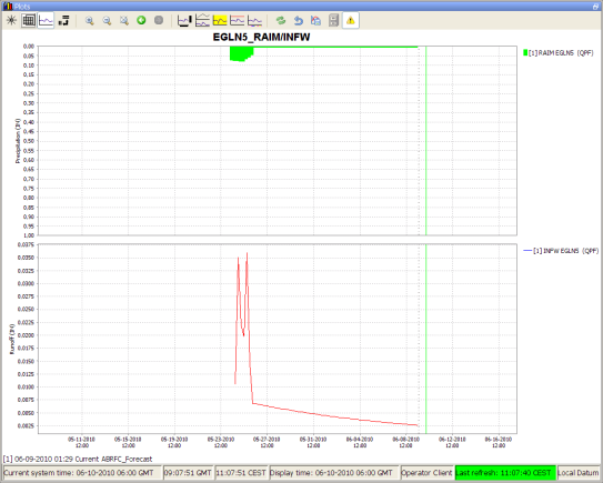
Inverted graphs
It is possible to invert the y-axis for a plot. This can be done by setting the inverted tag to true for a subplot.
Below is a configuration example
<display name="EGLN5_EGLN5">
<subplot>
inverted>true</inverted>
<plotWeight>1</plotWeight>
<timeSeriesSet>
<moduleInstanceId>FMAP_PreProcessing_QPF</moduleInstanceId>
<vlueType>scalar</valueType>
<parameterId>RAIM</parameterId>
<locationId>EGLN5</locationId>
<timeSeriesType>external forecasting</timeSeriesType>
<timeStep unit="hour" multiplier="6"/>
<relativeViewPeriod unit="hour" start="0" end="240"/>
<readWriteMode>editing visible to all future task runs</readWriteMode>
<synchLevel>5</synchLevel>
</timeSeriesSet>
</subplot>
ModifierTypes.xml
In the modifierTypes.xml we can define which kind of modifiers can be used in the interactive forecasting process. More information about this topic can be found in the chapter Modifiers.