This is an example of how to use the sealevel R package. This package is part of OpenEarth and available through r-forge for the convenience of R users. See Trends in Sea-Level Trend Analysis for a discussion on sea-level trend analysis.
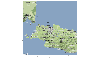
This example generates an overview of tide gauges near Jakarta and generates a plot of the measurements of the nearby stations.
|

|
# This is an example of how to get tide gauge data for Jakarta

library(sealevel) # the sealevel package
library(plyr) # reshape
library(ggplot2) # grammar of graphics
library(ggmap) # plot on top of googlemap

# get all the tide gauge data from PSMSL

# For Jakarta no revised local reference data is available.
# Please see the PSMSL site for details

# Get the url for the metric dataset
url <- get.psmsl.url(type='metric')

# Get the name of the file
path <- basename(url)
# Download all data (takes a while)
download.file(url, path)

# Read all monthly data
stations <- read.psmsl(path)

# Create an overview of all locations and names
stations.latlon <- ldply(stations, function(station){data.frame(lat=station$lat, lon=station$lon, name=station$name)})

# Plot a map of Jakarta
# 6.2S 106.8E
jakarta <- get_map(location = c(lon = 106.8, lat = -6.2), zoom = 8)
jakarta.map <- ggmap(jakarta)
# Plot the nearby tide gauges with the name as a lable
p <- jakarta.map + geom_point(data=stations.latlon, aes(x=lon, y=lat), color='red')  + geom_text(data=stations.latlon, aes(x=lon, y=lat, label=name), hjust=0.1, vjust=0.1, size=3)

# Save it to png
png('tidegaugemapjakarta.png', width=1000, height=600)
print(p)
dev.off()

# compute the distance from jakarta
dist <-  laply(stations, function(station){sqrt((station$lon - 106.8)**2 + (station$lat - -6.2)**2)})
# use the first 5 stations
jakarta.stations <- stations[order(dist)][1:10]
# combine them into 1 data fram
jakarta.df <- ldply(jakarta.stations, function(station) {df <- station$data; df$name <- station$name; df$waterlevel <- df$waterlevel - mean(df$waterlevel, na.rm=TRUE); return(df)})
# categorize by name
jakarta.df$name <- factor(jakarta.df$name)
# plot all gauges in one plot
jakarta.df$waterlevel <- jakarta.df$waterlevel + 100*as.numeric(jakarta.df$name)
p <- ggplot(jakarta.df, aes(year.month,waterlevel, color=name)) + geom_line() + geom_smooth() + labs(x='year', y='water level [mm]')

# Save it to png
png('tidejakarta.png', width=1000, height=600)
print(p)
dev.off()