02 Time Series Display Configuration

Introduction

The layout of the time series display is configured in an XML file in the System Configuration folder. When available on the file system, the name of the XML file is for example:

TimeSeriesDisplayConfig 1.00 default.xml

TimeSeriesDisplayConfig           Fixed file name for the time series display settings

1.00                                            Version number

default                                         Flag to indicate the version is the default configuration (otherwise omitted).

Figure 13 shows the main elements of the TimeSeriesDisplay configuration, These are divided into a number of sections, each of which will be discussed individually (these are indicated with a + sign).

Figure13 Elements in the TimeSeriesDisplay configuration

description

An optional description of the configuration. This is for reference purposes only and will not be used elsewhere.

General Display Configuration

This includes global setting for the time series display.

convertDatum

This optional Boolean setting can be used to start the time series display showing levels against the global reference level. The default is that levels are displayed against the local reference level. The difference between local and global reference is defined in the locations definition (see regional settings).

maximumInterpolationGap

Maximum gapsize which can be filled in by linear or block filler in the data editor

valueEditorPermission

Optional permission which must be assigned to a user to to edit values in the data editor

lableEditorPermission

Optional permission which must be assigned to a user to to edit labels in the data editor

commentEditorPermission

Optional permission which must be assigned to a user to to edit comments in the data editor

Default view period

The optional default view period can be used to define the time span of data displayed in the time series display (unless overruled by the user).

Parameters

• unit identifies the time unit with which the time span is defined (enumeration of second, minute, hour, day, week).
• start identifies the start time of the time span with reference to the T0 (in multiples of the unit defined).
• end identifies the start time of the time span with reference to the T0 (in multiples of the unit defined).

Time Markers Display Configuration

Time series display markers are informative lines in the display. These may be defined to display vertical lines for times values of interest. The configuration of horizontal threshold lines is also included in this definition. Markers can be defined for three time values as well as for the thresholds;

for time series

• systemTime
• displayTime
• timeZero
• threshold
• forecastConfidence1
• forecastConfidence2
• forecastConfidence3

Within longitudinal profile displays, the markers can be set to display the minimum or maximum values. A variety of river bed levels can be included in a display if these are specifed in the branches.xml file. 

for longitudinal profile:

• leftBankLevel
• leftFloodPlainLevel
• leftMainChannelLevel
• longitudinalProfileMaximum
• longitudinalProfileMinimum
• rightBankLevel
• rightFloodPlainLevel
• rightMainChannelLevel

To visualize model layer elevations when drawing a cross section in a spatial plot, one should use: bottomLayerLevel
topLayerLevelThis applies only for parameters with unit in meters

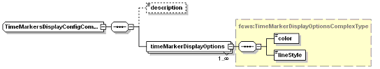
Figure 14 Elements in the TimeMarkersDisplay section of the TimeSeriesDisplay configuration

timeMarkerDisplayOptions

Root element of a definition time markers (multiple entries may exist).

Attributes;

• marker enumeration of the possible markers (see list above).

color

Colour of the time series marker line (see enumeration of colours in appendix A).

lineStyle

Line style of time series marker line. Enumeration of "solid", "none", "bar", "dashdot", "dashed", "dotted", "solid;thick", "dashdot;thick", "dashed;thick"; "dotted;thick"; "area"; "constant".

The "constant" label should preferably only be applied if the time series holds only one value.

label

Define the name of time series marker line.

Parameters display configuration

In this section of the time series display, default attributes of lines plotted for parameters can be allocated. These defaults will be used when plotting lines for these parameters in the time series displays and in the reports. Note that for allocation of the colour only the preferred colour can be identified. When the line is plotted this colour will be used only if there is no other line with the same colour. If this is the case then the next colour in the colour palette will be used.

Figure 15 Elements in the ParameterDisplayConfig section of the TimeSeriesDisplay configuration

PreferredColor

The preferred colour for the line and markers. This colour will only be used if it is not yet available in the current graph. If it is, then the next colour in the template order will be selected.

lineStyle

Line style of time series line. Enumeration of "solid", "none", "bar", "dashdot", "dashed", "dotted".

markerStyle

Marker style for markers plotted on the vertices of the line. Enumeration of "none", "+", "x", "circle", "square", "rectangle", "diamond", "triangleup" , "triangledown".

markerSize

Size of the marker in points

Precision

Decimal precision with which values are given in the table.

min

Minimum of the y-scale to be used as a default for all displays of this parameter. The minimum is used, unless a value in the time series is lower than this minimum, in which case that is used. The minimum defined here can also be overruled in individual template definition in the DisplayGroups (see below).

max

Maximum of the y-scale to be used as a default for all displays of this parameter. This maximum is used, unless a value in the time series is higher than this maximum, in which case that is used. The maximum defined here can also be overruled in individual template definition in the DisplayGroups (see below).

maxTimeSpan

Optional field, only intended to be used for viewing non-equidistant series. Specifying this value will prevent the drawing of line segments in the TimeSeriesDisplay between adjacent time/value points for which the time difference exceeds the specified maximum time span.

Module instance mapping

The module instance mapping allows user defined strings to be defined which will display the moduleInstanceID in the legends of the time series display. This can help shorten legends, or add additional information.

Figure 16 Elements in the Log Panel section of the Explorer configuration

moduleInstanceMapping

Root element for each mapping to be defined.

Attributes;

• id ModuleInstanceId to be replaced

description

String to replace the module instance id in the legends

Statistical functionality

Time series statistical functions are statistical functions that use one equidistant, scalar time series to produce another one using a statistical function. When defined, a list of statistical functions will be displayed in the Time Series Display. If the user selects a function then for each (equidistant, scalar) time series in the display another one is generated and displayed with the calculated results. Calculated time series are displayed in the same graph as the time series they are based on.

Some statistical functions require an additional accumulation time span, time step or samples which the user can select using a slider. As soon as the user selects a different value from the slider the calculation is launched with the new value.

The Statistical functions group defines dedicated graphing options shown in the combo box in the toolbar:

Calendar aggregation (with associated time step)

Creates an aggregation of a time series array according to the selected time step.

Attributes:

• function: calendarAggregation
• timeStep: Time steps that the user selects from using the slider.

Relative aggregation (with associated time span)

Creates an aggregation of a time series array. A relative time step is calculated by the selected time span and the start time of the period from the time series array.

Attributes:

• function: relativeAggregation
• movingAccumulationTimeSpan: Time spans that the user selects from using the slider.

Duration exceedence

Sorts the values in a time series array and its flags in descending order.

Attributes:

• function: durationExceedence

Duration non-exceedence

Sorts the values in a time series array and its flags in ascending order.

Attributes:

• function: durationNonExceedence

Moving average (with associated time span)

A moving average calculates the mean value of the all values within the selected time window.

Attributes:

• function: movingAverage
• ignoreMissings: when true, missing values are ignored and each average will be calculated from the available values within the current time window.
  When false, calculated values will be set to missing if one or more values within the current time window are missing.
• movingAccumulationTimeSpan: Time spans that the user selects from using the slider.

The moving average function only works for true equidistant data (i.e. no daysOfMonths etc.)
The difference between moving average and central moving average is that the central moving average uses values before and after the current value to calculate the average. Moving average only uses values in the past.

Central moving average (with associated time span)

A central moving average calculates the mean value of the time window of which the current value is in the middle. It is the same as the moving average, but shifted to the past for half the time window.

Attributes:

• function: centralMovingAverage
• ignoreMissings: when true, missing values are ignored and each average will be calculated from the available values within the current time window.
  When false, calculated values will be set to missing if one or more values within the current time window are missing.
• movingAccumulationTimeSpan: Time spans that the user selects from using the slider.

The central moving average function only works for true equidistant data (i.e. no daysOfMonths etc.)
The difference between moving average and central moving average is that the central moving average uses values before and after the current value to calculate the average. Moving average only uses values in the past.

Accumulation interval (with associated time span or time step)

The accumulation interval function creates cumulative series for several intervals. For the first output time step in each interval the output value equals the input value for that time step. For a given other output time step the output value is equal to the sum of the input value for that time step and the previous output value. The intervals are defined by the selected time span or the selected time step. If a time span is selected, then the function uses the time span as the size for the intervals and the first interval starts at the start of the period that is visible in the time series display. If a time step is selected, then the function uses the selected time step to create intervals. Each period between two consecutive time steps in the selected time step is an interval.

Attributes:

• function: accumulationInterval
• movingAccumulationTimeSpan: Time spans that the user can select using the slider.
  or
• timeStep: Time steps that the user can select using the slider.

Accumulation aggregation (with associated time span or time step)

The accumulation interval sums the values for all time steps within the selected time window range. The time window range is defined by the associated time span or time step.

Attributes:

• function: accumulationAggregation
• movingAccumulationTimeSpan: Time spans that the user can select using the slider.
  or
• timeStep: Time steps that the user can select using the slider.

Frequency distribution (with associated samples)

The frequencies of the available values are counted and are plotted within a number of bins to create a frequency distribution. The number of bins can be selected using the slider. The data range that is covered by the bins can be changed as follows. Clicking the "Set boundaries" button brings up the "Set boundaries" dialog. In this dialog the lowest bin boundary and the highest bin boundary can be changed. The space between these two boundaries is divided regularly into the selected number of bins. Initially the boundaries are in automatic mode. In automatic mode for each time series the minimum data value and the maximum data value are used as boundaries. When the user selects new boundaries manually, then the new boundaries will be used instead, i.e. manual mode. In manual mode the boundaries are fixed and the same boundaries are used for all time series, until they are changed again. This makes comparisons between different time series possible. When the user clicks the "Automatic" button, then the boundaries will be in automatic mode again.

In manual mode the selected boundaries are remembered. This means that when the user closes and re-opens the time series display or starts working in another separate time series display, then in manual mode the previously selected boundaries will still be used for new frequency distributions. The mode will also be the same for all time series displays.

Attributes:

• function: frequencyDistribution
• samples: The number of bins that the user can select using the slider.

Gaussian curve (with associated samples)

The mean value and standard deviation are calculated for the timeseries from which the normal distrubution function is calculated. The selected sample determines in how many samples the normal distribution function is divided into.

Attributes:

• function: gaussianCurve
• ignoreMissings: when true, missing values are ignored and each average will be calculated from the available values within the current time window.
  When false, calculated values will be set to missing if one or more values within the current time window are missing.
• samples: Definition of samples sizes that the user selects from using the slider.

Note: The displayed diagram is no longer a graph of unit time and therefore uses a different panel for displaying the graph. The associated tabel panel is currently not working for this type of graph and therefore the table toggle button will be disabled.

Show peaks above value

A scatterplot is made where the x-axis shows the duration of a 'peak' (=values within this peak-area are all above the given reference level), the y-axis shows the normalized difference between the parameter value and the reference level. The reference level can be altered by entering a value into the input field associated with this statistical function. After clicking 'Apply' the result time series array is returned.
If no reference level is entered, then the 'peak' areas are determined according to the minimum available value of the input time series array.

Attributes:

• function: showPeaksAbove

Show lows below value

A scatterplot is made where the x-axis shows the duration of a 'low' (=values within this low-area are all beneath the given reference level), the y-axis shows the normalized difference between the parameter value and the reference level. The reference level can be altered by entering a value into the input field associated with this statistical function. After clicking 'Apply' the result time series array is returned.
If no reference level is entered, then the 'low' areas are determined according to the maximum available value of the input time series array.

Attributes:

• function: showLowsBelow

Scatterplot

The data is displayed as a collection of points, each having the value of the timeseries determining the position on the horizontal axis and the value of the other timeseries (one or more) determining the position on the vertical axis.
The timeseries used for the horizontal- and vertical axis can be changed by the user by using the 'Series selection' dialog, which is opened by clicking on the 'Edit' button.

Attributes:

• function: scatterPlot

Note: The displayed diagram is no longer a graph of unit time and therefore uses a different panel for displaying the graph. The associated tabel panel is currently not working for this type of graph and therefore the table toggle button will be disabled.

Boxplot

The data is graphically displayed by a box-and-whisker diagram. The following five-number summaries are displayed: the smallest observation (sample minimum), lower quartile (Q1), median (Q2), upper quartile (Q3), and largest observation (sample maximum). An additional dot is plotted to represent the mean of the data in addition to the median.

Attributes:

• function: boxPlot

Note: The displayed diagram is no longer a graph of unit time and therefore uses a different panel for displaying the graph. The associated tabel panel is currently not working for this type of graph and therefore the table toggle button will be disabled.

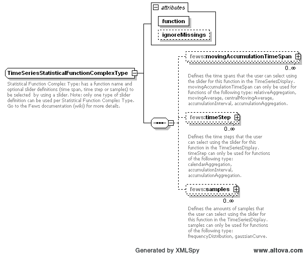
Schemas for the slider

movingAccumulationTimeSpan

Defines the time spans that the user can select using the slider for this function in the TimeSeriesDisplay. MovingAccumulationTimeSpan can only be used for functions of the following type: relativeAggregation, movingAverage, centralMovingAverage, accumulationInterval, accumulationAggregation.

timeStep

Defines the time steps that the user can select using the slider for this function in the TimeSeriesDisplay. TimeStep can only be used for functions of the following type: calendarAggregation, accumulationInterval, accumulationAggregation.

samples

Defines the amounts of samples that the user can select using the slider for this function in the TimeSeriesDisplay. Samples can only be used for functions of the following type: frequencyDistribution, gaussianCurve.

Descriptive Function Group

The descriptiveFunctionGroup defines the contents of the descriptive tabel. Several sub-table can be configured (see sample).

Functions supported are:

Info functions (if this type of function is specified, the display provides a hint to select a column in the table in order to get more descriptive information):

• info: displays parameter (long name+id), location (long name+id) 
• infoLocationId
• infoLocationName
• infoModuleinstance
• infoParameterId
• infoParameterName

Time series information available

• count: total number of populated records
• missings: total number of missings
• completed: number of records flagged as completed (gap filling)
• corrected: number of records flagged as corrected
• reliables: number of records flagged reliable
• unreliables: number of records flagged unreliable
• doubtfuls: number of recorsd flagged doubtfull

• startTime
• endTime

Descriptive statistical functions

The descriptive statistics functions are functions that are used for descriptive statistics. They can be defined to describe the distribution of the data (e.g. mean, min, max) or the data itself (info, start_time). All descriptive statistical functions produce a single value for a time series.

The descriptive functions results are displayed in group boxes that are named according to the group names that have been defined in the configuration file.

Attributes:
• function: Can be one of the functions below.
Information functions:

• info: Name of the time series
• start_time Start time of the time series in the view period
• end_time: End time of the time series in the view period
  Grouping functions:
• count: Number of time steps in the view period
• missings: Number of missing values in the view period
• doubtfuls: Number of doubtful values in the view period
• reliables: Number of reliable values in the view period
• unreliables: Number of unreliable values in the view period
  Statistical functions:
• mean: Mean value in the view period
• min: Lowest value in the view period
• max: Highest value in the view period
• percentile: Percentile in the view period for a given percentage (requires one or more value elements to define percentages; see below)
• standard_deviation: Standard deviation in the view period
• sum: Sum of the values in the view period
  • ignoreMissings: when true, missing values are ignored and each function will be calculated from the available values within the current time window.
  When false, calculated values will be set to missing if one or more values within the current time window are missing.

Duration curve

A duration curve illustrates the relationship between parameter values and their duration. When selected, the current graphs are replaced with duration curves.

Attributes:

• function: always duration.
• Moving average
  A moving average calculates the mean value of the time window directly before the current value.

Attributes:

• function: always moving_average.
• ignoreMissings: when true, missing values are ignored and each average will be calculated from the available values within the current time window.
  When false, calculated values will be set to missing if one or more values within the current time window are missing.

for more details, a Word-attachement is available.