01 Grid Display

Grid display

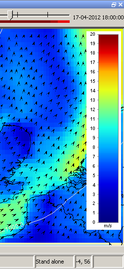
The grid display is used in DELFT-FEWS for viewing grid time series. These grid time series can be dynamically animated against a map background (comparable to the main map display).

The Id of the grid display is identified in the DisplayInstanceDescriptors. When available on the file system, the name of the XML file for configuring the GridDisplay with an Id of FloodMapDisplay is for example:

FloodMapDisplay 1.00 default.xml

Figure 143 Example of a configuration of the Grid Display

Besides plotting a grid in the grid display, it is also possible to plot scalar data (Figure 10) and longitudinal profiles (figure 9).

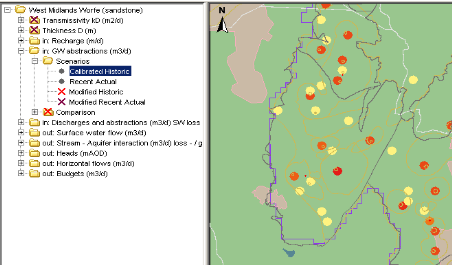
Figure 010 Example of a configuration of the scalar data in Grid Display

Figure 009 Example of a configuration of the longprofile in Grid Display

Figure 144 Root elements of the gridDisplay configuration

title

Name of the Grid Display. When opened this will appear in the title bar of the window.

defaults

Used to specify attributes that should apply to several gridPlots. Specifying which gridPlots the defaults apply to can be done through parameterGroupId, plotGroupId or plotId. When an attribute that is specified through defaults is needed, FEWS will search for the first defaults that contains the needed attribute and applies to the current gridPlot. If no parameterGroupId, no plotGroupId and no plotId is specified, the defaults is considered to apply to all gridPlots. Note that such a general defaults may override settings made in more specific defaults if it is found first by FEWS, when this occurs try specifying the most general defaults last. 

gridPlotGroup

Definition of a group in the grid display. Each group may have its own set of maps and time series to display. Defining groups creates a tree view in the left of the display (see example above). Multiple instances may exist.

Attributes;

• id : Id of the display group- this is used in the tree view.
• name : Optional name of the display group- used for reference purposes only

description

Optional description of the display group/grid plot. Used for reference purposes only

highlight

Optional property to highlight the Group name in bold in the selection filter.

gridPlot

Definition of a grid plot within the display group. Each grid plot forms a node in the tree view. When a gridPlot is selected, the appropriate maps will be displayed and the time series data retrieved from the database.

Attributes;

• id : Id of the grid plot- this is used in the tree view.
• name : Optional name of the grid plot- used for reference purposes only 
• contourlinescolor: required when the "contourlines button" in the griddisplay should be enabled

mapExtentId

Available since 2017.02. When the gridPlot is selected in the spatial display, the zoom extent will be automatically adapted to the specified extent. It is also possible to specify the mapExtentId for several gridPlots at once using the defaults. 

timeSeriesSet

Definition of the time series set to be displayed in the selected grid plot. This can refer to one location with valuetype grid or longitudinal profile, or it can refer to a locationSet of scalars. Contourlines can only be displayed in combination with a regular grid.

When 2D or 3D data is imported using multiple domain partitions, this data can be displayed using LocationSets. All partitions have a LocationId and a LocationSet can be created for reference to all partitions. This LocationSet can be used consistently throughout the gridDisplay configuration, like when displaying:

dataLayer

Use this option to display multiple data grids. Each grid will be displayed in a separate data layer. The layer specified last, will be shown on top.

If a layer contains scalar data (possibly with a locationSet for multiple locations), this will be converted to a grid to display in that layer showing data at the specified (point) locations as follows:

• timeSeriesSet: displayed as dots (see figure)
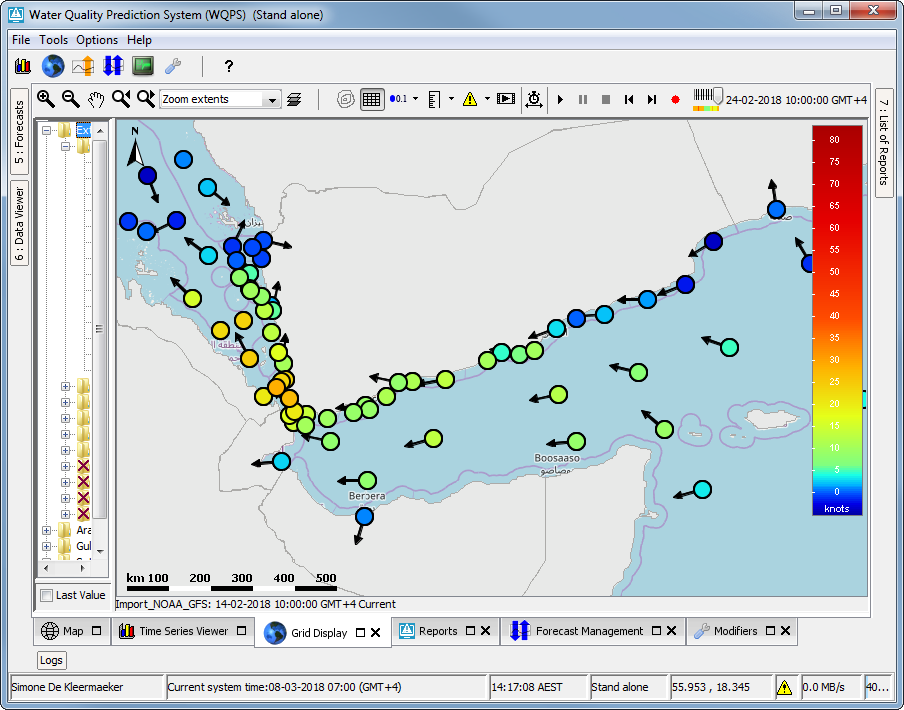
• uTimeSeriesSet and vTimeSeriesSet: displayed as arrows
• uTimeSeriesSet and vTimeSeriesSet, as well as a timeSeriesSet for the wind velocity for the same location(s): displayed as dots and arrows combined, resembling wind vanes (see figure)

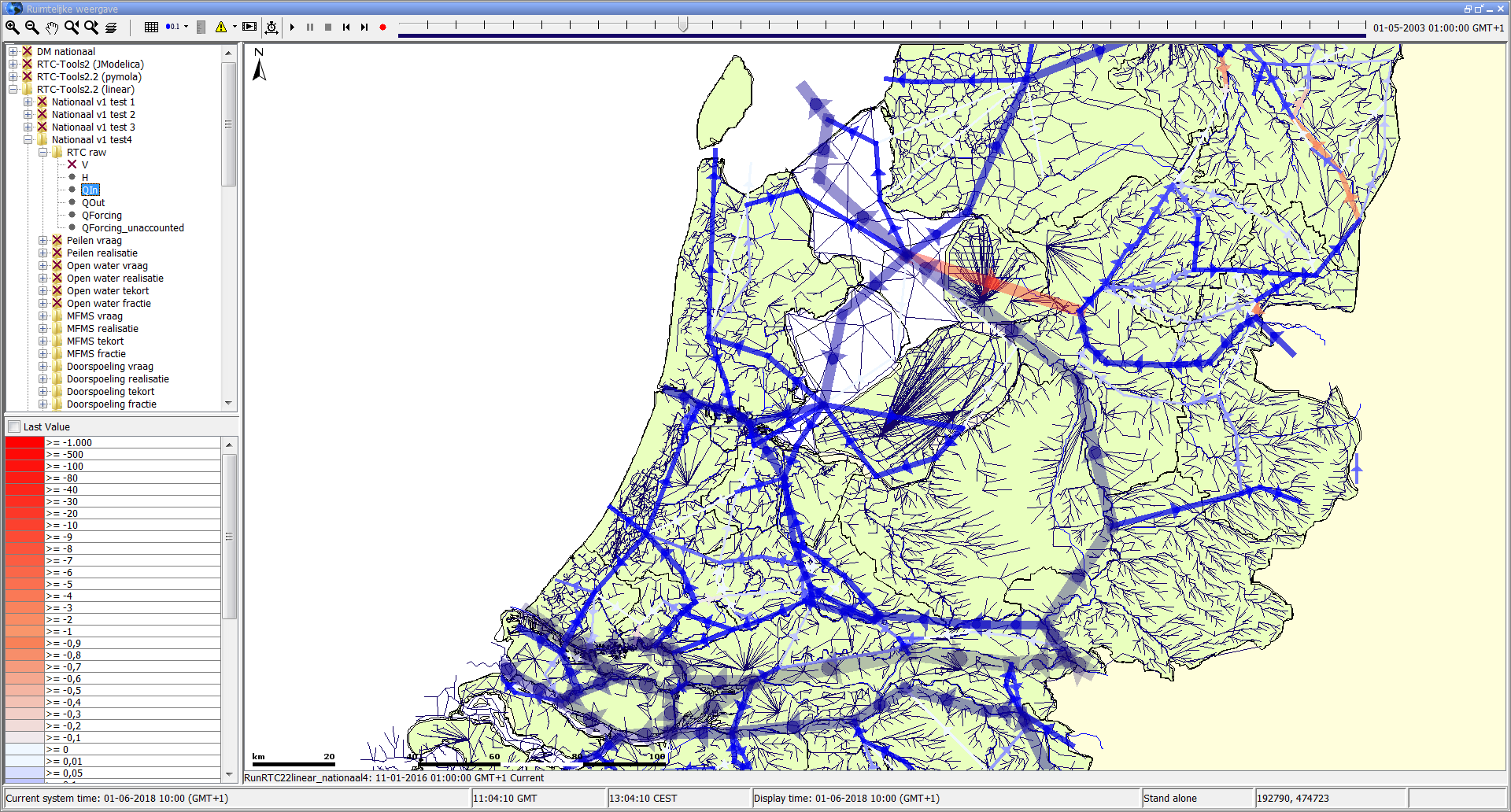
showArrowsOnLines

This element is available since 2018.01, in combination with a dataLayer containing a timeSeriesSet element. If this is set to true (false by default) and the locationSet in the timeSeriesSet contains (poly)-lines, the lines drawn in the spatial display will include directional arrows. If the time series has a positive value for a line, the arrow will point from the start of the line (first point found in the shape file) to the end of the line (second point found in the shape file). If the value is negative, the arrow is inverted. See the figures for examples.

showThumbnailsPanel

If this is true, then the grid display shows the spatial thumbnails panel when this grid plot is selected. Otherwise the grid display will not show the spatial thumbnails panel when this grid plot is selected. Default is false. After this grid plot has been selected, the user can still switch on/off the spatial thumbnails panel manually, using the toggle button in the grid display.

Since 2017.02, if this element is never configured for any grid plot, the user settings will be used to decide whether the thumbnails panels is shown on startup, and the panel will remain shown / hidden when a different grid plot is selected. If this element is configured for any grid plot, the thumbnails panel will always be hidden on startup, and actively shown / hidden when selecting a different grid plot depending on the configuration.

Before 2017.02, the user settings were never used to reinstate the status of the thumbnails panel on startup, the panel was always hidden. When selecting grid plots, the panel was shown / hidden depending on the configuration, until the user manually switches the panel on or off. Once a manual change was made, the panel remained shown / hidden even when selecting different grid plots for the remainder of the session. 

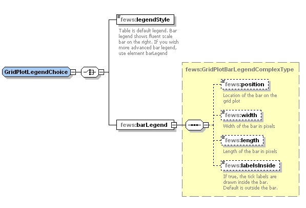
legendStyle

The legend can be shown as table legend or as bar legend.
Default legend style is table. Bar legend shows fluent scale bar on the right.

barLegend

Use this element to show customized bar legend.
The following legend properties can be changed:

• position: legend can be placed on the right, on the left, at the top or at the bottom. Default is on the right.
• width: width of the bar in pixels. Default is 40 pixels.
• length: length of the bar in pixels. The defaults are 400 for legend on the right/left, and  for the legend at the top/bottom the length equals the width of the window
• labelsInside: if true , ticks and labels are displayed inside the legend bar . The default is outside.

Elements of the configuration of legend style

valueTimeSeriesSet / directionTimeSeriesSet

If a timeseries with direction data is available, this is where the TimeSeriesSet should be placed. Note: a TimeSeriesSet with velocity values is required in the ValueTimeSeriesSet!

uTimeSeriesSet / vTimeSeriesSet

When data with velocities are available as a timeseries with the u-component and the v-component, these can be placed in the uTimeSeriesSet and vTimeSeriesSet elements. In the grid display automatically arrows will be drawn showing the direction, calculated on the v and u component. The velocity is presented in a color, defined in the classBreaks.

Double clicking in the grid display will open the u and v timeseries in the timeseries display. If one of the following is configured, they will be opened instead:

• Adding the uvAmplitudeParameterId element (since 2015.02), where an amplitude parameter can be configured, the timeseries display will combine the u and v timeseries into one amplitude timeseries (sqrt(u^2+v^2)).
• Adding the uvDirectionParameterId element (since 2016.01), where a wind direction parameter can be configured, the timeseries display will combine the u and v timeseries into one wind direction timeseries. The wind direction is in degrees, where the north direction is 360 degrees, east is 90 degrees, south is 180 degrees and west is 270 degrees. 

uvAmplitudeParameterId (since 2015.02)

Id of a parameter that corresponds to the amplitude of this u,v data (e.g. wind speed). If this amplitude parameter is configured and the user double clicks on a grid cell in the grid display, then the TimeSeriesDialog will only display the amplitude sqrt(u^2+v^2) of this u,v data. The displayed amplitude time series uses the configured amplitude parameter. If neither the uvAmplitudeParameterId nor the uvDirectionParameterId is configured, then the TimeSeriesDialog only displays the separate u and v time series.

uvDirectionParameterId(since 2016.01)

Id of a parameter that corresponds to the direction of this u,v data (e.g. wind direction). If this direction parameter is configured and the user double clicks on a grid cell in the grid display, then the TimeSeriesDialog will only display the direction. The displayed wind direction time series uses the configured direction parameter. If neither the uvAmplitudeParameterId nor the uvDirectionParameterId is configured, then the TimeSeriesDialog displays the separate u and v time series.

uvDirectionParameterConvention (since 2016.02)

Configure the direction of arrows drawn in the grid display. Options are:

• to, typically used when displaying flow data or
• from, typically used when displaying wind data - this is the default option, which is used when nothing is configured.

sigmaScaleReferenceTimeSeriesSet (since 2017.02)

Additional timeSerieSet to link the sigma layers in a 3D model to indexed layers. For this you also need a locationSet linking a parentLocation to all sigma layers. Each sigma layer is linked to an index in a MapLayerFile. The parentLocation needs to be defined in Location.xml, linked to a grid definition in Grids.xml. See for a full config example Sigmalayers - display D-FlowFM 3D results in GridDisplay.

Accumulation / Moving Average slider or Last Value Checkbox

Optionally, an accumulation or moving average slider can be configured. If this slider is present the last value checkbox, is shown by default, which can optionally be hidden. Only one of the following elements may be configured, although the chosen element may appear several times when configuring a slider:

• <movingAverageTimeSpan>: When configured a slider is displayed with the configured time spans. If a time span is selected in the slider, then the data in the grid display is aggregated (moving average) using that time span. The start of a timeSpan is exclusive and the end of a timeSpan is inclusive. Configure a very large time span (eg 100000 days) to allow the user to see the total average of the loaded time series.
• <movingAccumulationTimeSpan>: When configured an accumulation slider is displayed with the configured time spans. If a time span is selected in the slider, then the data in the grid display is aggregated (moving accumulation) using that time span. The start of a timeSpan is exclusive and the end of a timeSpan is inclusive. Configure a very large time span (eg 100000 days) to allow the user to see the total sum of the loaded time series.
• <accumulationTimeSpan>: Since 2014.02. When configured an accumulation slider is displayed with the configured time spans. When a time span is selected with the slider, the interval of the ticks in the time slider in the grid display is recalculated to the selected time step. Configure a very large time span (eg 100000 days) to allow the user to see the total sum of the loaded time series.
• <accumulationTimeStep>: Since 2016.02. When configured an accumulation slider is displayed with the configured time steps. When a time step is selected with the slider, the interval of the ticks in the time slider in the grid display is recalculated to the selected time step. Configure a very large time step (eg 100 years) to allow the user to see the total sum of the loaded time series.
• <hideLastValueCheckBox>: Since 2017.02. Default false. When set to true, the "show last value" will be hidden. Note that if an accumulation slider is configured, the checkbox will be hidden by default.

Config example for configuring a moving accumulation time span slider:

<gridPlot id="MeteoSat">
	<!-- omitted the time series configuration for clarity -->
	<movingAccumulationTimeSpan unit="hour" multiplier="6"/>
	<movingAccumulationTimeSpan unit="hour" multiplier="12"/>
	<movingAccumulationTimeSpan unit="day" multiplier="1"/>
	<movingAccumulationTimeSpan unit="day" multiplier="2"/>
	<movingAccumulationTimeSpan unit="day" multiplier="3"/>
</gridPlot>

verticalSliderRange (since 2017.02)

When a sigmaScaleReferenceTimeSeriesSet is configured, a vertical slider becomes automatically visible in GridDisplay to slide through the water column, displaying the 2D model results at a arbitrary water depth. The values displayed are dynamically interpolated between the sigma layers of the model, but only for the visible time step for performance reasons.  The range of the slider is automatically adjusted to all available water depths for whole period, however you can limit this range using the <verticalSliderRange> option. See for a config example Sigmalayers - display D-FlowFM 3D results in GridDisplay.

geoMap

Definition of the maps used as a background to the dynamic grid displayed. The layout and zoom extent are also defined in this element. More information on the configuration of the geoMap element can be found here.

classBreaks

Definition of colors to use in displaying the dynamic grid. These are also shown in the legend on the left of the grid display (see example elsewhere on this page). Optional when default class breaks are available for this plot group and parameter group.

Figure 145 Elements of the configuration of class breaks

description

Optional description. Since FEWS 2017.01 it is allowed to have multiple class breaks for a plot. The user can switch between the class breaks with a drop down list. This description is used in the drop down list.

missingValueColor

Color that is used to display missing values (NaN values) for point locations and tracks. Default is fully transparent.

missingValueOpaquenessPercentage

Opaqueness percentage that is used to display missing values (NaN values) for point locations and tracks. This overrules the opaqueness of the configured missingValueColor. If missingValueOpaquenessPercentage is not configured, then opaqueness of missingValueColor is used

unitVisible (available since build 18734)

When this is true the display unit for the class break values will be displayed in the legend. Default is false. The display unit can be configured in parameter group.

rescaleAroundOrdinalValue (available since build 17892)

Definition of the optional ordinal value that will always keep the same colour when the class break colours are rescaled in the grid display. After rescaling, the highest lowerValue will be changed to the maximum grid value visible in the current zoom extent and the lowest lowerValue will be changed to the minimum grid value visible in the current zoom extent. The lowerValues and the colours in between will be rearranged to fit between the minimum and maximum. Thus the colours for given values change.
If no ordinal value is specified, then the colours are just rearranged. However, if e.g. ordinal value = 0 is specified and 0 values have a white colour, then the rescaling will take this into account so that 0 values always stay coloured white. This can be used for instance when displaying temperatures, where red colours are used for positive values and blue colours are used for negative values and zero values are coloured white.

lowerColor

Colour definition for the colour in the legend associated with the lowest value in the range.

upperColor

Colour definition for the colour in the legend associated with the highest value in the range.

lowerOpaquenessPercentage

Optional definition of the opaqueness of the colour in the legend associated with the lowest value in the range.

upperOpaquenessPercentage

Optional definition of the opaqueness of the colour in the legend associated with the highest value in the range.

lowerSymbolSize

Optional definition of the size of symbols associated with the lowest value in the range.

upperSymbolSize

Optional definition of the size of symbols associated with the highest value in the range.

lowerValue

Definition of the value at which the colour in the grid displayed changes. The legend will be a gradual change in colours from the lowest colour to the highest colour, with the number of increments determined by the number of lowerValue items entered. Multiple entries may exist.

color

Deprecated, use break.

break

The options described above can be used for definitions of lowerValues that have colors that change gradually between a lowerColor and upperColor. The break option can be used instead for specifying a discrete lowerValue with an absolute color, symbolSize and opaquenessPercentage. In this case, set colorSmoothingEnabled to false. Multiple entries may exist. Labels cannot contain the ">" and "<" sign. To present these, use the  &gt; and &lt; respectively.

geoMap (or background maps)

The background maps to be displayed are defined in the geoMap element. More information on the configuration of the geoMap element can be found here. 

Extracting data from the Spatial Display

The user can create plots on the fly based on the data presented in the Spatial display. Depending on the data this can be:

• scalar time series
• longitudinal profile
• 2D longitudinal profile
• data for an area from a grid time series
• data for multiple plots at once
• save and loading sketches 

This all explained in the user Delft-FEWS User Guide: 05 Spatial Display

Configuration (Examples)

The following example shows how to configure a Meteosat image as grayScaleImage in the Grid display.

<gridPlotGroup id="Meteosat Images">
	<gridPlot id="MeteoSat">
		<timeSeriesSet>
			<moduleInstanceId>ImportMeteosat</moduleInstanceId>
			<valueType>grid</valueType>
			<parameterId>image</parameterId>
			<locationId>meteosat</locationId>
			<timeSeriesType>external historical</timeSeriesType>
			<timeStep unit="minute" multiplier="15"/>
			<relativeViewPeriod unit="hour" start="-12" end="36"/>
			<readWriteMode>read only</readWriteMode>
		</timeSeriesSet>
		<classBreaks>
			<lowerColor>black</lowerColor>
			<upperColor>white</upperColor>
			<lowerValue>0</lowerValue>
			<lowerValue>8</lowerValue>
			<lowerValue>16</lowerValue>
			<lowerValue>24</lowerValue>
			<lowerValue>32</lowerValue>
			<lowerValue>40</lowerValue>
			<lowerValue>48</lowerValue>
			<lowerValue>56</lowerValue>
			<lowerValue>64</lowerValue>
			<lowerValue>72</lowerValue>
			<lowerValue>80</lowerValue>
			<lowerValue>88</lowerValue>
			<lowerValue>96</lowerValue>
			<lowerValue>104</lowerValue>
			<lowerValue>112</lowerValue>
			<lowerValue>120</lowerValue>
			<lowerValue>128</lowerValue>
			<lowerValue>136</lowerValue>
			<lowerValue>144</lowerValue>
			<lowerValue>152</lowerValue>
			<lowerValue>160</lowerValue>
			<lowerValue>168</lowerValue>
			<lowerValue>176</lowerValue>
			<lowerValue>184</lowerValue>
			<lowerValue>192</lowerValue>
			<lowerValue>200</lowerValue>
			<lowerValue>208</lowerValue>
			<lowerValue>216</lowerValue>
			<lowerValue>224</lowerValue>
			<lowerValue>232</lowerValue>
			<lowerColor>orange</lowerColor>
			<upperColor>red</upperColor>
			<lowerValue>240</lowerValue>
			<lowerValue>248</lowerValue>
			<lowerValue>255</lowerValue>
		</classBreaks>
	</gridPlot>
</gridPlotGroup>

3D data display (example)

The following example shows how to configure 3D data originating from several computational domains in the Grid display.

<gridPlot id="3D_data" name="3D data display">
    <dataLayer>
        <arrowColor>white</arrowColor>
        <arrowSymbol>flow</arrowSymbol>
        <multipleArrowsPerValue>false</multipleArrowsPerValue>
        <uTimeSeriesSet>
            <moduleInstanceId>DFlowFM_FC</moduleInstanceId>
            <valueType>grid</valueType>
            <parameterId>C.simulated.u</parameterId>
            <locationSetId>DFlowFM_0_####</locationSetId>
            <timeSeriesType>simulated forecasting</timeSeriesType>
            <timeStep unit="nonequidistant"/>
            <readWriteMode>read complete forecast</readWriteMode>
        </uTimeSeriesSet>
        <vTimeSeriesSet>
            <moduleInstanceId>DFlowFM_FC</moduleInstanceId>
            <valueType>grid</valueType>
            <parameterId>C.simulated.v</parameterId>
            <locationSetId>DFlowFM_0_####</locationSetId>
            <timeSeriesType>simulated forecasting</timeSeriesType>
            <timeStep unit="nonequidistant"/>
            <readWriteMode>read complete forecast</readWriteMode>
        </vTimeSeriesSet>
        <uvAmplitudeParameterId>C.simulated.speed</uvAmplitudeParameterId>
        <uvDirectionParameterId>C.simulated.dir</uvDirectionParameterId>
        <sigmaScaleReferenceTimeSeriesSet>
            <moduleInstanceId>DFlowFM_FC</moduleInstanceId>
            <valueType>grid</valueType>
            <parameterId>WD.simulated</parameterId>
            <locationSetId>DFlowFM.merged</locationSetId>
            <timeSeriesType>simulated forecasting</timeSeriesType>
            <timeStep unit="nonequidistant"/>
            <readWriteMode>read complete forecast</readWriteMode>
        </sigmaScaleReferenceTimeSeriesSet>
    </dataLayer>
 
    <barLegend>
        <position>right</position>
        <width>50</width>
        <length>400</length>
        <labelsInside>true</labelsInside>
    </barLegend>
    <classBreaksId>Class.Currents</classBreaksId>
    <contourLinesColor>antique white</contourLinesColor>
</gridPlot>

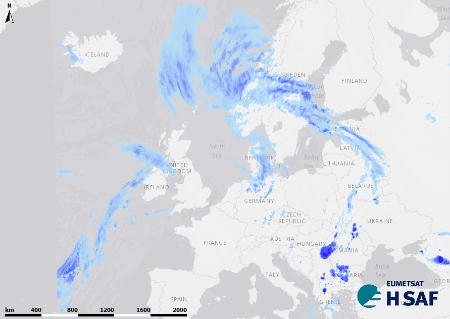
Logo at map

Some satelite products require to be shown with a logo, where the imageFile with the logo should be located in the MaplayerFiles directory.

The logo file can be place at the next positions: topLeft, bottomLeft, topRight or bottomRight.

<gridPlot id="Precipitation">
	<timeSeriesSet>
		<moduleInstanceId>Import_NWP</moduleInstanceId>
		<valueType>grid</valueType>
		<parameterId>P.fc</parameterId>
		<qualifierId>aladin_hr</qualifierId>
		<locationId>NWP_ALADIN_HR</locationId>
		<timeSeriesType>external forecasting</timeSeriesType>
		<timeStep unit="hour"/>
		<relativeViewPeriod unit="day" start="-5" end="10"/>
		<readWriteMode>read only</readWriteMode>
	</timeSeriesSet>
	<logo>
		<imageFile>logo.png</imageFile>
		<position>topRight</position>
	</logo>
	<classBreaksId>Precipitation_1h</classBreaksId>
	<contourLinesColor>gray</contourLinesColor>
</gridPlot>