1 General description

1.1 Introduction

The urban water balance tool (Figure 1) has been developed in EXCEL for application in urban area. Recently it has been transformed into a set of Python scripts. The water balance tool describes all possible urban water flows and the associated water resources. Rainfall-runoff, shallow groundwater (saturated and unsaturated), surface water and sewage (both mixed and stormwater drainage) are included. Water exchanges are included with atmosphere, deep groundwater, outside water and waste water treatment plant.

Figure 1 Schematic overview of Urbanwb model

In this figure:

Elements		Water flows
A	= area	P_atm	= precipitation
atm	= atmosphere	E_atm	= evaporation
PR	= paved roof	T_atm	= transpiration
CP	= closed paved	R_up	= decoupled runoff
OP	= open paved	R_ow	= runoff to open water
UP	= unpaved	I_uz	= infiltration
OW	= open water	P_gw	= percolation
UZ	= unsaturated zone	D_ow	= drainage
GW	= groundwater	S_out	= downward seepage
MSS	= mixed sewer system	R_mss / R_swds	= runoff to sewer systems
SWDS	= stormwater drainage system	SOF	= sewer overflow on street
SO	= sewer overflow	Q_ow	= discharge to open water
WWTP	= waste water treatment plant	Q_out	= discharge to outside / WWTP

History

Originally the time step was 1 day. That way time series of more than 100-year rainfall and evaporation could be managed in EXCEL. A smaller time step could also be applied (1 hour, 15 minutes, 5 minutes). However, because of the limitations of EXCEL, a smaller time step implies much shorter time series. Transforming the water balance tool to a set of Python scripts solved this limitation. This set of Python scripts that has been combined in the Urbanwb model. This documentation describes the Urbanwb model.

Model purpose

This tool has been developed to determine the return periods of runoff events for relatively small urban areas in which the basic hydro(geo)logic conditions are assumed to be similar for the entire area. Determination of runoff return periods requires large time series of rainfall and evaporation, preferably at least 30 years.

The calculation results of the Urbanwb model are much less accurate and detailed as the calculation results of detailed hydraulic models, like SOBEK and MIKE-urban. It is commonly accepted to design urban water systems based on the calculation results of these hydraulic models for a single design rainstorm. However, the runoff caused by a design rainstorm, also depends on the initial conditions in all parts of the urban water system.

Main advantage of the Urbanwb model is that multiple different rainstorms with all kinds of actual antecedent weather conditions, resulting in all kinds of different initial conditions in all parts of the urban water system, are calculated. Other relevant advantages are that both model building and model calculations take much less time.

General model description

The Urbanwb model is a lumped conceptual model for urban water balance modelling. Urbanwb model simulates dominant dynamic hydrological processes of an urban water system. Rainfall-runoff processes, shallow groundwater (saturated and unsaturated zone), surface water and sewer systems (mixed and stormwater drainage) are all incorporated in Urbanwb model. Three external boundaries are included (atmosphere, deep groundwater and outside water / waste water treatment plant) to where water can be exchanged.

Figure 1 provides a schematic overview of Urbanwb model with its fundamental elements included. Under this conceptual framework, major hydrological dynamics in an urban water system can be quickly and indicatively modelled to provide users with a general idea of the water quantity distribution and how the water system behaves under certain conditions.

Below you find a brief introduction of the major components of the Urbanwb model. Chapter 2 describes these components into much more detail.

1.2 Major components

In the Urbanwb, the land use area is divided into:

Paved area above floor level
o Paved Roof (PR), i.e. buildings.
Paved area at floor level
o Closed Paved (CP), completely sealed.
o Open Paved (OP), allowing some infiltration.
Unpaved area at floor level
o Unpaved (UP).
Surface water at floor level
o Open Water (OW).

Below floor level, the distinguished components are:

Unsaturated Zone (UZ)
o Since water is assumed to flow mainly vertically in the UZ is irrelevant below PR and CP from where all runoff flows directly into the sewer system (SWDS, MSS) or to UP when defined disconnected. UZ is neither relevant below OP where the limited infiltration is assumed percolating directly into GW. In other words, UZ is only relevant below UP areas for plant transpiration.
Shallow groundwater (GW)
o Although theoretically possible, UZ is assumed to be not present beneath OW. That implies that the groundwater level is irrelevant below OW, though the model allows to define a certain percentage of OW to be above the phreatic water table. The same goes for the groundwater below PR where a percentage of PR above groundwater level can be defined. Conversion of water flows between reservoirs with different areas depends on the area ratio of these reservoirs.
Sewer system (MSS and SWDS)
o    A mixed sewer system (MSS) collects stormwater and domestic (and industrial) wastewater in the same pipe system. In extreme rain conditions, untreated mixed sewer overflows may cause serious pollution to recipient water bodies (Figure 2).

Figure 2      Mixed sewer system under dry, wet weather conditions, source: Wikipedia.
o    Storm water drainage system (SWDS), i.e. the stormwater drainage component of two separate sewer systems. Separate sewer systems overcome the drawback of sewer overflow pollution of combined sewer system through disposing wastewater and stormwater into two separate systems. The storm water drainage system module is incorporated in the Urbanwb model

Boundaries, over which external water exchanges occur, are:

Atmosphere (Atm)
o Rainfall and potential evapo(transpi)ration are the main driving forces in the Urbanwb. Since the Urbanwb is a simple lumped conceptual model, other factors like temperature, relative humidity, wind and solar radiation are irrelevant. However solar radiation can be applied during preprocessing to transform daily evaporation time series into time series with smaller time steps.
Deep groundwater (Deep GW)
o Seepage from shallow groundwater (GW) to deep groundwater can be defined in the Urbanwb, either as a constant flux (downward, upward or zero) or as a dynamically computed water flow dependent on the difference between the computed groundwater level and the defined hydraulic head of the deep groundwater and on the defined vertical flow resistance.
Outside water and waste water treatment plant (Out and WWTP)
o MSS discharges its water to WWTP. The excess water in OW, i.e. water above target water level, is discharged to Outside Water. Both outflows are limited by predefined discharge rates. When the water level in OW get below the target water level, the difference is supplied by Outside Water (negative discharge).
Note
A typical Dutch polder has no natural gradient for drainage, thus excessive water is normally pumped through a pumping station into a higher elevated network of larger primary canals (Figure 3) from where the water is released into sea at low tide.

Figure 3 Dutch polder system, source: Hum 300 The Arts in Society.

1.3 General assumptions

Only rainfall is considered as the precipitation. Rainfall is instantaneously at the beginning of each time step.
Rainfall is intercepted by the surface layer, from where for paved areas first evaporation occurs and then (for open paved areas) infiltration for that time step starts. The evaporation rate is limited by the potential open water evaporation for that time step and infiltration is limited by the infiltration capacity of the open paved area. In unpaved areas evaporation and infiltration empty the interception storage simultaneously.
The runoff from paved areas flow to the sewer systems regardless of their inflow capacities (exceedance of this capacity is dealt with separately as sewer overflow on the street). Runoff from disconnected paved areas flows to the unpaved area.
All relevant parameters are defined by users in accordance with local conditions for the project area, like land use, soil, vegetation, surface water level, etc. Detailed explanations on parameter input is in chapter 2.
Calculated water flows and storage volumes are all expressed in depth (mm) per area for that component. For reservoir B, inflow from reservoir A to B is converted from outflow from A by considering the area ratio of reservoir A over B. For example, area of A is 5m², area of B is 10m², calculated outflow from A to B in terms of A is 2mm/hr, then the inflow of B from A in terms of B is 2 × = 1mm/hr. In Urbanwb model, the water quantity is strictly conserved not only for the individual reservoir but also for the entire model.
Internal routing is irrelevant in Urbanwb model. It takes no time for the water to “travel” between reservoirs. Consequently, the model is applicable at neighbourhood scale and use at large spatial scale may be questionable. An analogy would be a glass of water being knocked over with water spilling over the table instantly, i.e. the mass balance is conserved but routing is ignored.
Urban adaptation measures can be implemented with Urbanwb model through incorporating Adaptive Measure module. The measure module is an individual component that interacts with the basic reservoirs of Urbanwb model. Detailed explanations on adaptive measure structure is described in section 2.9 .
Parameters to initialize the model are allocated into two parts and saved in separate configuration files. In the neighbourhood configuration file, parameters of local urban environment like land use fractions, soil type, target water level, etc. are stored. In the measure configuration file, parameters to that setup the measure are stored. Since for any model goes “Garbage in = garbage out”, we advise the user to estimate model parameters based on scientific literature and empirical evidence supported by expert judgement.
Any water flow from A to B (e.g. infiltration) is basically limited by three aspects: the available water volume in A, the available storage in B and the transport capacity from A to B.

2 Model components

This section explains in detail how each of the Urbanwb components is architected. Their underlying principles, simplifying assumptions, and calculation orders are explained in depth in this section. At the end of this chapter, in section 2.9 , the method of applying adaptation measures is described. The possibility of generating runoff to adaptation measures however, is provided in all components.

2.1 Paved Roof

Paved Roof (PR) refers to all kinds of buildings in an urban area ranging from low-rise buildings (e.g. single dwelling, apartment complex) to high-rise buildings (e.g. high-rise housing, skyscraper). On rooftop, a roof drainage system collects rainwater in gutters and drains it into a sewer through a downspout pipe. A small amount of rainwater ponded or intercepted on the roof surface is defined as interception storage. It can be emptied only through evaporation. Water exceeding the interception storage capacity becomes runoff on the Paved Roof. Basically, all runoff ends in the sewer system (SWDS and/or MSS). However, the Urbanwb offers the option of disconnecting (part of) the runoff. The disconnected part of the runoff is assumed to flow to the Unpaved area. Figure 4 provides a schematic overview.

Figure 4 Schematic overview of Paved Roof (PR) in Urbanwb

2.1.1 Assumptions

Rainwater falling on the building roof is first retained as interception storage and depleted by evaporation, and then excess water becomes runoff. In other words, only rainfall exceeding interception storage capacity runs off. Provided that a considerably large interception storage capacity on Paved Roof is predefined, there is no runoff generated.
(Connected) runoff on Paved Roof is redistributed to sewer systems (SWDS and MSS) and Unpaved (UP) by predefined ratios. If part of roof is disconnected to sewer system, for instance a minor fraction of water flows out from the roof edge down to the ground directly, that disconnected fraction of runoff is assumed to flow to Unpaved area. However, given a normally functioning roof drainage system, the majority of the runoff from Paved Roof contributes to the storm water drainage system (SWDS) or (and) combined sewer system (MSS) at predefined proportions.

2.1.2 Calculation order

Initial interception storage on Paved Roof at the beginning of current time step is remaining interception storage on Paved Roof at the end of previous time step plus rainfall at current time step, and it is limited by predefined interception storage capacity on Paved Roof.
(Actual) evaporation from interception on Paved Roof during current time step is limited by potential Open Water evaporation and available initial interception storage on Paved Roof during the same time step. Evaporation is possible only if the interception storage contains water.
(Final) interception storage on Paved Roof at the end of current time step is evaporation subtracted from initial interception storage.
(Total) runoff from Paved Roof during current time step is rainfall subtracting actual evaporation and the change in interception storage between the same time step and previous time step. Total runoff from Paved Roof are redistributed to the measure (Meas), sewer system (SWDS and MSS) and Unpaved (UP) at predefined ratios.
Subtracting the runoff to the measure from total runoff is the remaining runoff. Connected remaining runoff is reallocated to storm water drainage system (SWDS) and combined sewer system (MSS) at predefined proportions while disconnected remaining runoff flows to Unpaved area (UP) at predefined ratio.

2.1.3 Code and input arguments

class urbanwb.pavedroof.PavedRoof(intstor_pr_t0, pr_no_meas_area, pr_meas_area, pr_meas_inflow_area, intstorcap_pr=1.6, swds_frac=1.0, discfrac_pr=0.0, **kwargs) [source]

Bases: _object

Creates an instance of PavedRoof class with given initial states and properties, iterates sol() function to compute states and fluxes of Paved Roof at each time step.

Parameters:

intstor_pr_t0 (float) – initial interception storage on Paved Roof (at t=0) [mm]
r_no_meas_area (float) – area of Paved Roof without measure [m^2]
pr_meas_area (float) – area of Paved Roof with measure [m^2]
pr_meas_inflow_area (float) – measure inflow area from Paved Roof, i.e. runoff inflow area to measure from Paved Roof (>= area of Paved Roof with measure and <= total area of Paved Roof) [m^2]
intstorcap_pr (float) – predefined interception storage capacity on Paved Roof [mm]
swds_frac (float) – part of urban paved area with storm water drainage system (SWDS) [-]
discfrac_pr (float) – part of Paved Roof that is disconnected from sewer system [-]

inflowfac() [source]

Calculates measure inflow factor of Paved Roof.

Returns: Measure inflow factor of Paved Roof

inflowfac – measure inflow factor is calculated as (runoff inflow area to measure from Paved Roof - area of Paved Roof with measure) / area of Paved Roof without measure

Return type: (float)

sol(p_atm, e_pot_ow) [source]

Calculates states and fluxes on Paved Roof during current time step.

Parameters:

p_atm (float) – rainfall during current time step [mm]
e_pot_ow (float) – potential Open Water evaporation during current time step [mm]

Returns: A dictionary of computed states and fluxes of Paved Roof during current time step

int_pr – Interception storage on Paved Roof after rainfall at the beginning of current time step [mm]
e_atm_pr – Evaporation from interception storage on Paved Roof during current time step [mm]
intstor_pr – Remaining interception storage on Paved Roof at the end of current time step [mm]
r_pr_meas – Runoff from Paved Roof to measure during current time step (not necessarily on Paved Roof itself) [mm]
r_pr_swds – Runoff from Paved Roof to storm water drainage system (SWDS) during current time step [mm]
r_pr_mss – Runoff from Paved Roof to combined sewer system (MSS) during current time step [mm]
r_pr_up – Runoff from Paved Roof to Unpaved during current time step [mm]

Return type: (dictionary)

2.2 Closed Paved

Closed Paved areas are mainly areas with paved covers like roads, parking lots, driveways, etc. that are made of impermeable material like cement and bituminous concrete pavement. In terms of conceptual modelling mechanisms, Closed Paved is quite similar to Paved Roof. On the surface of a typical impermeable paved area, a small amount of rainwater is intercepted as surface ponding which can only be emptied through evaporation. Rainfall exceeding the interception storage capacity will generate runoff, which flows to the sewer system (SWDS and/or MSS). The disconnected fraction of runoff is assumed to flow to the Unpaved area (UP). Figure 5 provides a schematic overview.

Figure 5 Schematic overview of Closed Paved (CP) in Urbanwb

2.2.1 Assumptions

Rainwater falling on the Closed Paved is first ponded as surface interception storage and depleted by evaporation, then the excessive rainwater becomes runoff. In other words, only rainfall exceeding the interception storage capacity runs off. Provided that a very large interception storage capacity on Closed Paved is predefined, there is no runoff generated.
Runoff on the Closed Paved is redistributed to sewer system (SWDS and MSS) and Unpaved (UP) by predefined ratios. If part of Closed Paved area is disconnected to the sewer system, that disconnected fraction of runoff flows to Unpaved area by assumption. Connected runoff on Closed Paved flows to the storm water drainage system (SWDS) or (and) combined sewer system (MSS) at predefined proportions.

2.2.2 Calculation order

Initial interception storage on Closed Paved at the beginning of current time step is the remaining interception storage on Closed Paved at the end of previous time step plus rainfall at current time step, and it is limited by predefined interception storage capacity on Closed Paved.
(Actual) evaporation from interception on Closed Paved during current time step is limited by potential Open Water evaporation and available initial interception storage on Closed Paved during the same time step. Evaporation is possible only if the interception storage contains water.
(Final) interception storage on Closed Paved at the end of current time step is evaporation subtracted from initial interception storage.
(Total) runoff from Closed Paved during current time step is rainfall subtracting actual evaporation and the change in interception storage between the same time step and previous time step. Total runoff from Closed Paved is redistributed to the measure (Meas), sewer system (SWDS and MSS) and Unpaved (UP) at predefined ratios.
Subtracting the runoff to the measure from the total runoff is the remaining runoff. Connected remaining runoff is reallocated to storm water drainage system (SWDS) and combined sewer system (MSS) at predefined proportions while disconnected remaining runoff flows to Unpaved area (UP) at predefined ratios.

2.2.3 Code and input arguments

class urbanwb.closedpaved.ClosedPaved(intstor_cp_t0, cp_no_meas_area, cp_meas_area, cp_meas_inflow_area, intstorcap_cp=1.6, swds_frac=1.0, discfrac_cp=0.0, **kwargs) [source]

Bases: _object

Creates an instance of ClosedPaved class with given initial states and properties, iterates sol() function to compute states and fluxes of Closed Paved at each time step.

Parameters:

intstor_pr_t0 (float) – initial interception storage on Closed Paved (at t=0) [mm]
pr_no_meas_area (float) – area of Closed Paved without measure [m^2]
cp_meas_area (float) – area of Closed Paved with measure [m^2]
cp_meas_inflow_area (float) – measure inflow area from Closed Paved, i.e. runoff inflow area to measure from Closed Paved (>= area of Closed Paved with measure and <= total area of Closed Paved) [m^2]
intstorcap_cp (float) – predefined interception storage capacity on Closed Paved [mm]
swds_frac (float) – part of urban paved area with storm water drainage system (SWDS) [-]
discfrac_cp (float) – part of Closed Paved that is disconnected from sewer system [-]

inflowfac() [source]

Calculates measure inflow factor of Closed Paved.

Returns: Measure inflow factor of Closed Paved

inflowfac – measure inflow factor is calculated as (runoff inflow area to measure from Closed Paved - area of Closed Paved with measure) / area of Closed Paved without measure

Return type: (float)

sol(p_atm, e_pot_ow) [source]

Calculates states and fluxes on Closed Paved during current time step.

Parameters:

· p_atm (float) – rainfall during current time step [mm]
· e_pot_ow (float) – potential Open Water evaporation during current time step [mm]

Returns: A dictionary of computed states and fluxes of Closed Paved during current time step

int_cp – Interception storage on Closed Paved after rainfall at the beginning of current time step [mm]
e_atm_cp – Evaporation from interception storage on Closed Paved during current time step [mm]
intstor_cp – Remaining interception storage on Closed Paved at the end of current time step [mm]
r_cp_meas – Runoff from Closed Paved to measure during current time step (not necessarily on Closed Paved itself) [mm]
r_cp_swds – Runoff from Closed Paved to storm water drainage system (SWDS) during current time step [mm]
r_cp_mss – Runoff from Closed Paved to combined sewer system (MSS) during current time step [mm]
r_cp_up – Runoff from Closed Paved to Unpaved during current time step [mm]

Return type: (dictionary)

2.3 Open Paved

Open Paved areas are paths, sidewalks, parking area and other less imperviously paved areas that have relatively limited infiltration capacity. These somewhat permeable pavements use porous material that allows water flowing through it (e.g. pervious concrete, porous asphalt) or spaced nonporous material (e.g. paving stones, permeable interlocking concrete pavement) that allows water infiltrate between the cracks (Figure 6 ). Consequently, compared to the Paved Roof (PR) and Closed Paved (CP) components, the Open Paved (OP) component has an extra infiltration flux from Open Paved surface to groundwater. This infiltration flux is limited by an infiltration capacity as well as by the available interception storage on the Open Paved area. Rainfall exceeding the interception storage capacity will generate runoff, which flows to the sewer system (SWDS and/or MSS). The disconnected fraction of runoff is assumed to flow to the Unpaved area (UP). Figure 7 provides a schematic overview.

Figure 6 Permeable pavement — porous asphalt and interlocking pavement, source: google images.

Figure 7 Schematic overview of Open Paved (OP) in Urbanwb

2.3.1 Assumptions

On Open Paved, cracks on the pavement and pores in the material that allow infiltration only occupy a very minor fraction of Open Paved surface area. Hence it does not affect the interception storage capacity on Open Paved surface.
Infiltration starts after interception storage is filled and it is limited by predefined infiltration capacity. Interception storage can only be emptied through evaporation.
There is no vegetation on the Open Paved area, and consequently no transpiration from root zone below the surface. Hence, for simplicity, the infiltration from Open Paved surface is directly percolating into the groundwater (GW) and passes the Unsaturated Zone.

2.3.2 Calculation order

Initial interception storage on Open Paved at the beginning of current time step is the remaining interception storage on Open Paved at the end of previous time step plus rainfall at current time step, and it is limited by predefined interception storage capacity on Open Paved.
(Actual) evaporation from interception on Open Paved during current time step is limited by potential Open Water evaporation and available initial interception storage on Open Paved during the same time step. Evaporation is possible only if the interception storage contains water.
(Final) interception storage on Open Paved at the end of current time step is evaporation subtracted from initial interception storage.
The infiltration (percolation to groundwater) occurs only if interception storage gets fully filled. Infiltration is limited by predefined infiltration capacity on Open Paved. Infiltration directly flows to groundwater (GW), i.e. percolation (skipping Unsaturated Zone).
(Total) runoff from Open Paved during current time step is rainfall subtracting actual evaporation, the change in interception storage between the same time step and previous time step and percolation to groundwater. Total runoff is redistributed to the measure (Meas), storm water drainage system (SWDS), combined sewer system (MSS) and Unpaved (UP) at predefined ratios.
Subtracting runoff to the measure from total runoff is the remaining runoff. Connected remaining runoff is reallocated to storm water drainage system (SWDS) and combined sewer system (MSS) at predefined proportions, whilst disconnected remaining runoff flows to Unpaved area (UP) at predefined ratio.

2.3.3 Code and input arguments

class urbanwb.openpaved.OpenPaved(intstor_op_t0, op_no_meas_area, op_meas_area, op_meas_inflow_area, intstorcap_op=1.6, infilcap_op=1.0, swds_frac=1.0, discfrac_op=0.0, **kwargs) [source]

Bases: _object

Creates an instance of OpenPaved class with given initial states and properties, iterates sol() function to compute states and fluxes of Open Paved at each time step.

Parameters:

intstor_pr_t0 (float) – initial interception storage on Closed Paved (at t=0) [mm]
intstor_op_t0 (float) – initial interception storage on Open Paved (at t=0) [mm]
op_no_meas_area (float) – area of Open Paved without measure [m^2]
op_meas_area (float) – area of Open Paved with measure [m^2]
op_meas_inflow_area (float) – measure inflow area from Open Paved, i.e. runoff inflow area to measure from Open Paved (>= area of Open Paved with measure and <= total area of Open Paved) [m^2]
intstorcap_op (float) – predefined interception storage capacity on Open Paved [mm]
infilcap_op (float) – predefined infiltration capacity on Open Paved [mm/d]
swds_frac (float) – part of urban paved area with storm water drainage system (SWDS) [-]
discfrac_op (float) – part of Open Paved that is disconnected from sewer system [-]

inflowfac() [source]

Calculates measure inflow factor of Open Paved.

Returns: measure inflow factor of Open Paved

inflowfac – measure inflow factor is calculated as (runoff inflow area to measure from Open Paved - area of Open Paved with measure) / area of Open Paved without measure

Return type: (float)

sol(p_atm, e_pot_ow, delta_t) [source]

Calculates states and fluxes on Open Paved during current time step.

Parameters:

p_atm (float) – rainfall during current time step [mm]
e_pot_ow (float) – potential Open Water evaporation during current time step [mm]
delta_t (float) – length of time step [d]

Returns: A dictionary of computed states and fluxes of Open Paved during current time step

int_op – Interception storage on Open Paved after rainfall at the beginning of current time step [mm]
e_atm_op – Evaporation from interception storage on Open Paved during current time step [mm]
intstor_op – Remaining interception storage on Open Paved at the end of current time step [mm]
p_op_gw – Percolation from interception storage on Open Paved to groundwater during current time step [mm]
r_op_meas – Runoff from Open Paved to measure during current time step (not necessarily on Open Paved itself) [mm]
r_op_swds – Runoff from Open Paved to storm water drainage system (SWDS) during current time step [mm]
r_op_mss – Runoff from Open Paved to combined sewer system (MSS) during current time step [mm]
r_op_up – Runoff from Open Paved to Unpaved during current time step [mm]

Return type: (dictionary)

2.4 Unpaved

Unpaved area is a land use type that has no paved surface cover, e.g. gardens and grassland, on which the water can much more easily infiltrate than on paved surface. Vegetation (crop) type on the Unpaved area needs to be predefined. The model assumes notable distinction between paved areas (PR, CP and OP) and unpaved areas (UP). From paved areas, excess water is mainly drained through the sewer system. From unpaved areas, excess water mainly infiltrates to the unsaturated zone underneath, percolates to the groundwater and is drained via groundwater flow to the drainage system (open water). Rainfall water stored in the interception layer at the surface simultaneously evaporates to the atmosphere and infiltrates to Unsaturated Zone. Water exceeding the interception storage capacity is assumed to runoff to Open Water (OW). Figure 8 provides a schematic overview.

Figure 8 Schematic overview of Unpaved (UP) in Urbanwb

2.4.1 Assumptions

Disconnected runoff from paved area is equally spread over the Unpaved area. This runoff is added to the water available for infiltration and evaporation.
The interception capacity on Unpaved area is defined as the water depth above which surface runoff generates. Interception capacity of vegetation is not separately defined. Evaporation by the vegetation is taken up in the transpiration from Unsaturated Zone (UZ). Evaporation and infiltration from the Unpaved surface will occur as long as water remains on surface level.
Infiltration starts after (initial) interception storage contains water. (Initial) interception storage is proportionally emptied by infiltration and evaporation. The excessive part from interception storage capacity becomes runoff. Infiltration is limited by actual infiltration capacity and available storage in the Unsaturated Zone. Evaporation is limited by the potential open water evaporation during that time step. Infiltration and evaporation during a times step occur simultaneously and are limited by the available initial interception storage.
Actual infiltration capacity during current time step is limited by the actual available free space in the Unsaturated Zone, i.e. the maximum moisture content minus the actual moisture content in root zone during the same time step. However, the anticipated percolation from Unsaturated Zone to Groundwater during the same time step allows more infiltration. The anticipated percolation is limited by the saturated permeability of the soil and the available water for percolation.
A defined Time factor is that part of the time step that water is remaining on surface level. Potential Open Water evaporation is multiplied with this time factor to get the actual evaporation of the Unpaved area for that time step. The actual infiltration capacity is multiplied with this time factor to get the actual infiltration from the Unpaved area to the Unsaturated Zone for that time step.
Rainwater falling on Unpaved areas together with runoff from disconnected paved area is first intercepted as (initial) surface interception storage and emptied by evaporation and infiltration, then the excessive rainwater becomes runoff. In other words, only rainfall exceeding the interception storage capacity runs off. Provided that a considerably large interception storage capacity on Unpaved areas is predefined, there is no runoff generated.
Except runoff from UP to measure when defined possible, all other runoff water on Unpaved flows to Open Water (OW) by assumption. If no Open Water area is present, the water cannot runoff and will be stored on the surface of Unpaved. In that case the water can only evaporate or infiltrate. However, for current version Urbanwb Model, the possibility of no Open Water presence has not yet been fully investigated and tested. Hence, to avoid potential errors, we advise to specify non-zero fraction for Open Water (OW).

2.4.2 Calculation order

Total runoff from disconnected paved area to Unpaved is the sum of runoff from disconnected paved area (PR, CP, OP) to Unpaved area (UP) after conversion with the area ratio.
(Initial) interception storage on Unpaved land at the beginning of current time step is the final remaining interception storage at the end of previous time step plus precipitation at current time step plus total runoff from disconnected paved area. It is not limited by interception storage capacity because (initial) interception storage is a transient variable which is only relevant in computing process.
(Actual) infiltration capacity during current time step is limited by predefined infiltration capacity of Unpaved and available free space in root zone for infiltration. Available free space in Unsaturated Zone for infiltration is limited by maximum moisture content of the root zone minus moisture content of soil at previous time step plus anticipated percolation during current time step. Anticipated percolation is limited by the saturated permeability of the soil and the available water for percolation.
As stated in assumptions, the time factor is that part of the time step that water is remaining on the surface level. Hence the time factor during current time step is limited by 1 and the ratio of initial interception storage over the sum of potential evaporation and actual infiltration capacity during current time step. With the time factor, actual evaporation and actual infiltration can be determined proportionally.
(Actual) evaporation during current time step is potential evaporation multiplied by the time factor.
(Actual) infiltration from Unpaved to Unsaturated Zone during current time step is actual infiltration capacity multiplied by the time factor.
(Final) interception storage on land is limited by the predefined interception storage capacity on Unpaved land and initial interception storage on land subtracting actual evaporation and actual infiltration.
(Total) runoff on Unpaved land during current time step is part of the (initial) interception storage after evaporation and infiltration still exceeding predefined interception storage capacity on Unpaved. Total runoff is redistributed to the measure (Meas) and Open Water (OW). When inflow runoff from Unpaved to measure defined possible, part of runoff flows to the measure according to predefined ratio, whilst the rest runoff from Unpaved land flows to Open Water (OW) by assumption.

2.4.3 Code and input arguments

class urbanwb.Unpaved.Unpaved(fin_intstor_up_t0, up_no_meas_area, up_meas_area, up_meas_inflow_area, intstorcap_up=20, infilcap_up=48, soiltype=2, croptype=1, **kwargs) [source]

Bases: _object

Creates an instance of Unpaved class with given initial states and properties, iterates sol() function to compute states and fluxes of Unpaved at each time step.

Parameters:

fin_intstor_up_t0 – initial final remaining interception storage on Unpaved (at t=0) [mm]
up_no_meas_area (float) – area of Unpaved without measure [m^2]
up_meas_area (float) – area of Unpaved with measure [m^2]
up_meas_inflow_area (float) – measure inflow area from Unpaved, i.e. runoff inflow area to measure from Unpaved (>= area of Unpaved with measure and <= total area of Unpaved) [m^2]
intstorcap_up (float) – predefined interception storage capacity on Unpaved [mm]
infilcap_up (float) – predefined infiltration capacity on Unpaved [mm/d]
soiltype (int) – soil type
croptype (int) – crop type

inflowfac() [source]

Calculates measure inflow factor of Unpaved.

Returns: measure inflow factor of Unpaved

inflowfac – measure inflow factor is calculated as (runoff inflow area to measure from Unpaved - area of Unpaved with measure) / area of Unpaved without measure

Return type: (float)

sol(p_atm, e_pot_ow, r_pr_up, r_cp_up, r_op_up, theta_uz_prevt, pr_no_meas_area, cp_no_meas_area, op_no_meas_area, ow_no_meas_area, delta_t=0.041666666666666664) [source]

Calculates states and fluxes on Unpaved during current time step.

Parameters:

p_atm (float) – rainfall during current time step [mm]
e_pot_ow (float) – potential Open Water evaporation during current time step [mm]
r_pr_up (float) – runoff from Paved Roof to Unpaved during current time step [mm]
r_cp_up (float) – runoff from Closed Paved to Unpaved during current time step [mm]
r_op_up (float) – runoff from Open Paved to Unpaved during current time step [mm]
theta_uz_prevt (float) – moisture content of root zone at previous time step [mm]
pr_no_meas_area (float) – area of Paved Roof without measure [m^2]
cp_no_meas_area (float) – area of Closed Paved without measure [m^2]
op_no_meas_area (float) – area of Open Paved without measure [m^2]
ow_no_meas_area (float) – area of Open Water without measure [m^2]
delta_t (float) – length of time step [d]

Returns: A dictionary of computed states and fluxes of Unpaved during current time step

sum_r_up – Sum of runoff from all paved areas to Unpaved during current time step [mm]
init_intstor_up – Initial interception storage on Unpaved after rainfall at the beginning of current time step [mm]
actl_infilcap_up – Actual infiltration capacity on Unpaved during current time step [mm]
mefac_up – Time factor, i.e. part of time step that interception storage on Unpaved is available for infiltration and evaporation during current time step [-]
e_atm_up – Evaporation from interception storage on Unpaved during current time step [mm]
i_up_uz – Infiltration from interception storage on Unpaved to Unsaturated Zone during current time step [mm]
fin_intstor_up – Final remaining interception storage on Unpaved at the end of current time step [mm]
r_up_meas – Runoff from Unpaved to measure during current time step (not necessarily on Unpaved itself) [mm]
r_up_ow – Runoff from Unpaved to Open Water during current time step [mm]

Return type: (dictionary)

2.5 Unsaturated Zone

Underneath Unpaved areas (UP) is an Unsaturated Zone (UZ). The Unsaturated Zone, often called the vadose zone, is the portion of the subsurface above the groundwater table. As mentioned before the Urbanwb does not apply an Unsaturated Zone in paved areas (PR, CP and OP), thus by assumption the Unsaturated Zone has the same area size as the Unpaved area. Infiltration from the Unpaved surface is an inflow to the Unsaturated Zone and percolation from the Unsaturated Zone to the groundwater (GW) is an outflow. In the Unsaturated Zone, we focus on the root zone from where the plant transpiration take place as the water uptake through plant roots. The root zone can be represented by means of a container in which the water content may fluctuate. Rainfall infiltration and capillary rise of groundwater towards the root zone add water to the root zone and decrease root zone depletion, while soil evaporation, crop transpiration and percolation removes water from root zone and increase depletion (Allen et al, 1998). Evapotranspiration the from root zone is modelled as the product of reference crop evapotranspiration (using Penman-Monteith evaporation or Makkink evaporation) and transpiration reduction coefficient (Panman, 1948; Montheith, 1965). Transpiration reduction coefficient is derived from the concept of Feddes plant water stress factor in the literature (Feddes et al, 1978).

Figure 9 shows the schematic overview of the Unsaturated Zone. Two important definitions are recapped here. Field capacity is the amount of water that a well-drained soil can hold against gravitational forces. In the absence of water supply, the water content in the root zone decreases as result of water uptake by the crop. As water uptake progresses, the remaining water is held to the soil particles with greater force, lowering its potential energy and making it more difficult for the plant to extract it. Eventually, the so called wilting point is reached where the crop can no longer extract the remaining water in the soil and the water uptake becomes zero. The wilting point is the soil water content at which plants will permanently wilt.

Figure 9 Schematic overview of Unsaturated Zone (UZ) in Urbanwb

Figure 10 shows how the transpiration reduction factor is related to soil water pressure head h (i.e. root zone water potential). In the range between h₃ (transpiration reduction point) and h₂ (field capacity), root water uptake is optimal (maximal), so the transpiration reduction factor α= 1.

When h < h₃, there is drought stress, and α linearly reduces to zero at h₄ (wilting point).

When h > h₂, α linearly reduces to zero at h₁ (fully saturated, i.e. anoxic moisture condition).

The threshold pressure h₃ increases with potential transpiration rates, i.e. daily crop-evaporation. For low potential transpiration rate, the threshold pressure h_3l is lower than the threshold pressure h_3h at high potential transpiration rate. Computational simplifications are made here to calculate daily crop-evaporation value. Evaporation data are often provided on daily basis. When the Urbanwb model is applied for smaller time steps (Δt), we derive the hourly values of h₃ based on the daily evaporation values by divided by 2Δt, where Δt is expressed in days (e.g. Δt = 1 hour = 1/24 day). The factor 2 is applied, based on the assumptions that evapotranspiration mainly occurs during day time and that day time lasts on average 12 hours.

Figure 10 Transpiration reduction coefficient in Urbanwb (i.e. plant water stress factor) in relation to root zone water potential. Source: Dejongvanlier et al, 2008.

Some applied concepts regarding evapotranspiration based on literature are:

Evapotranspiration: Evapotranspiration is an important component of the water cycle and is composed of two-subprocesses: evaporation from soil and vegetation surfaces and transpiration from plant through root-stomata system. Evaporation and transpiration occur simultaneously and there is no easy way of distinguishing between the two processes.
Reference crop evapotranspiration ET₀: The evapotranspiration rate from a reference surface, not short of water, is called reference crop evapotranspiration or reference evapotranspiration and is denoted as ET₀. The reference surface is a hypothetical grass reference crop with an assumed crop height of 0.12 m, a fixed surface resistance of 70 s/m and an albedo of 0.23. As a result of an Expert Consultation held in May 1990, the FAO Penman-Monteith method is recommended as the sole standard method for the definition and computation of the reference crop evapotranspiration method for determining ET₀. ET₀ can also be estimated from pan evaporation. Pans have proved their practical value and have been used successfully to estimate ET₀ by observing the water loss from the pan and using empirical coefficients to relate pan evaporation to ET₀. However, special precautions and management must be applied. Besides, Makkink evaporation commonly used in the Netherlands can be used to estimate ET₀ as well. Makkink evaporation = 0.8982 * Penman Monteith evaporation according to STOWA (2009).
Crop evapotranspiration under standard conditions ET_c: The crop evapotranspiration under standard conditions, denoted as ET_c, is the evapotranspiration from disease-free, well fertilized crops, grown in large fields, under op mum soil water conditions, and achieving full production under the given climatic conditions. ET_c= K_cET₀.
K_c is the crop factor (crop coefficient). The effect of both crop transpiration and soil evaporation are integrated into this single crop coefficient K_c. K_c varies with crop type, growth stage and other factors, the range of which is commonly (0.2 < K_c< 1.3). For simplicity, we say that the crop factor K_c= 1 for a hypothetical grass reference crop.
(Actual) evapotranspiration ET: As stated above, the ET from crop surfaces under standard conditions is determined by a crop coefficient K_c that relates ET_c to ET₀. However, actual evapotranspiration is usually under non-standard conditions. The ET from crop surfaces under non-standard conditions is adjusted by a water stress coefficient (α) and/or by modifying the crop coefficient. Hence, the (actual) evapotranspiration is ET = α ∗ K_c∗ ET₀. In the Urbanwb model, we take 1.0 for crop factor, Penman-Monteith evaporation (or Makkink evaporation) for reference crop evapotranspiration, transpiration reduction factor as water stress factor, so the modelled evapotranspiration is ET = α ∗ 1 ∗ E_PM.
Makkink evapotranspiration: Though Penman-Monteith method is solely recommended by FAO to calculate reference crop evapotranspiration and has been commonly used world widely, there are several other methods popular in certain area or nations. Makkink method is named after Gerrit François Makkink, a Dutch hydrologist (Makkink, 1957). The Makkink method is simple but must be calibrated to a specific location. Since 1987, the national Dutch Weather services KNMI used Makkink method as standard method to calculate reference crop evapotranspiration. Hence, Makkink evaporation can be used as the forcing “reference crop evapotranspiration” and can replace of Penman-Monteith evaporation, especially for study cases in the Netherlands. The relationship between Makkink evaporation and Penman-Monteith evaporation is Makkink evaporation = 0.8982 * Penman-Monteith evaporation according to STOWA (2009).

2.5.1 Assumptions

Infiltration from the Open Paved surface (OP) percolates directly to groundwater (GW) without passing Unsaturated Zone. Unsaturated Zone is only relevant beneath Unpaved area. The area of Unsaturated Zone is equal to area of the Unpaved area.
Since the Urbanwb model is evaluated for smaller time steps Δt than a day (currently Δt = 1 hour), for computing simplicity, hourly reference crop evapotranspiration is divided by 2Δt to get the daily crop-evaporation value as the potential transpiration rate that determines the transpiration reduction point h₃. The factor 2 (in 2 Δt) is applied, because it is assumed that (crop-)evaporation occurs only during day time (half a day). Actually, it would be better to apply the sum of hourly reference crop evapotranspiration for 24 hourly time steps within that day as the daily crop evaporation value, but for the sake of computing efficiency and robustness, we use this simplification and we argue this simplification is a good approximation and has negligible impacts on computed results.
(Actual) evapotranspiration during current time step is determined by transpiration reduction factor (water stress factor) and reference crop evapotranspiration during the same time step (crop factor =1).
Percolation to groundwater is limited by the saturated conductivity of the soil.

2.5.2 Calculation order

Total infiltration from Unpaved area is taken as the influx.
Calculate runoff from measure to Unsaturated Zone if defined possible.
Calculate moisture content of soil in the root zone at transpiration reduction point θ_h3. If daily reference evapotranspiration is less than 1 mm/d, θ_h3= θ_h3l. If daily reference evapotranspiration is more than 5 mm/d, θ_h3= θ_h3h. If daily reference evapotranspiration is between 1 mm/d and 5 mm/d, θ_h3 is interpolated between θ_h3l and θ_h3h.
Determine transpiration reduction factor α by linear interpolation between θ_h1 (moisture content of root zone at complete saturation point), θ_h2 (moisture content of root zone at field capacity), θ_h3 (moisture content of root zone at transpiration reduction point), and θ_h4(moisture content of root zone at permanent wilting point), based on actual moisture content of root zone at previous time step plus the infiltration from Unpaved area during current time step.
Evapotranspiration from Unsaturated Zone during current time step is the product of transpiration reduction factor α and reference crop evapotranspiration ET₀ during the same time step.
Determine equilibrium root zone moisture content θ_eq by interpolation, based on the groundwater level at previous time step. In database, for given soil type and crop type, we have information on equilibrium moisture content of root zone for different groundwater levels (from 0 to 10 m-SL). Hence, the equilibrium moisture content of root zone during current time step θ_eq is interpolated from the lookup table based on the groundwater level at previous time step.
Determine maximum capillary rise by interpolation, based on the groundwater level at the previous time step. In database, for given soil type, we have information on maximum capillary rise for different groundwater levels (from 0 to 10 m-SL). Similarly, to calculating equilibrium moisture content of root zone, the maximum capillary rise during current time step is interpolated from the lookup table based on the groundwater level at previous time step.
Determine percolation from Unsaturated Zone (UZ) to groundwater (GW). It can be positive (downward deep percolation) and negative (upward capillary rise). Note that deep percolation to groundwater and capillary rise from water table are summarized into one term in the Urbanwb model. If current root zone water budget (root zone moisture content at previous time step + infiltration from UP + runoff from measure to UZ - evapotranspiration) is greater than equilibrium root zone moisture content θ_eq, it is downward deep percolation, otherwise it is upward capillary rise. Deep percolation is limited by saturated permeability of the soil and difference between current water budget and equilibrium root zone moisture content θ_eq; Capillary rise is limited by maximum capillary rise and different between current water budget and equilibrium root zone moisture content θ_eq.
Determine moisture content of root zone θ at the end of current time step. The root zone moisture content at the end of current time step is the root zone moisture content at the end of previous time step + infiltration + runoff from measure – evapotranspiration percolation, which values are all calculated above.

2.5.3 Code and input arguments

class urbanwb.unsaturatedzone.UnsaturatedZone(theta_uz_t0, uz_no_meas_area, uz_meas_area, soiltype=2, croptype=1, **kwargs) [source]

Bases: _object

Creates an instance of UnsaturatedZone class with given initial states and properties, iterates sol() function to compute states and fluxes of Unsaturated Zone at each time step.

Parameters:

theta_uz_t0 (float) – initial (volumetric) moisture content of soil in the root zone (at t=0) [mm]
uz_no_meas_area (float) – area of Unsaturated Zone without measure [m^2]
uz_meas_area (float) – area of Unsaturated Zone with measure [m^2]
soiltype (int) – soil type
croptype (int) – crop type

sol(i_up_uz, meas_uz, e_ref, tot_meas_area, gwl_prevt, delta_t=0.041666666666666664) [source]

Calculates states and fluxes in Unsaturated Zone during current time step.

Parameters:

i_up_uz (float) – infiltration from interception storage on Unpaved to Unsaturated Zone during current time step [mm]
meas_uz (float) – inflow from measure to Unsaturated Zone during current time step [mm]
e_ref (float) – reference crop evapotranspiration during current time step [mm]
tot_meas_area (float) – total area of measure [m^2]
gwl_prevt (float) – groundwater level at previous time step [m-SL]
delta_t (float) – length of time step [d]

Returns: A dictionary of computed states and fluxes of Unsaturated Zone during current time step:

sum_i_uz – Infiltration from Unpaved to Unsaturated Zone during current time step [mm]
r_meas_uz – Inflow from measure (if applicable) to Unsaturated Zone during current time step [mm]
theta_h3_uz – Moisture content of root zone at which transpiration reduction starts during current time step [mm]
t_alpha_uz – Transpiration reduction factor during current time step [-]
t_atm_uz – Transpiration from Unsaturated Zone during current time step [mm]
gwl_up – First value in predefined lookup table above the groundwater level at the end of previous time step [m-SL]
gwl_low – First value in predefined lookup table below the groundwater level at the end of previous time step [m-SL]
theta_eq_uz – Equilibrium moisture content of root zone during current time step [mm]
capris_max_uz – Maximum capillary rise in root zone during current time step [mm/d]
p_uz_gw – Percolation from Unsaturated Zone to groundwater during current time step (positive: deep percolation, negative: capillary rise) [mm]
theta_uz – Moisture content of root zone at the end of current time step [mm]

Return type: (dictionary)

2.6 Groundwater

In the Urbanwb Model, underneath the Unsaturated Zone is the saturated zone, i.e. the Groundwater reservoir (GW). The Groundwater reservoir is modelled as an unconfined aquifer which consists of a pervious layer underlain by a (semi-)impervious layer, below which lies the deep groundwater, one of the boundary components that exchanges water with the Urbanwb model. Percolation from Unsaturated Zone and Open Paved recharges the groundwater, while downward seepage to deep groundwater and drainage to Open Water deplete the Groundwater reservoir. The inflow (percolation from Unsaturated Zone) and outflow (seepage and drainage) are driven by the head difference, so the value of these fluxes can both be positive or negative. Figure 11 shows the schematic overview of the Groundwater reservoir. The area of the Groundwater reservoir is calculated as the area of the total model minus the area of Open Water fraction that is not above the groundwater level and minus the area of Paved Roof fraction of which the basement is below groundwater. The maximum capillary rise and the storage coefficient for the current time step are determined by interpolation based on the groundwater level at the end of the previous time step.

Figure 11 Schematic overview of groundwater reservoir (GW) in Urbanwb

The formula of groundwater level during current time step h(t) and its derivation are shown below (Figure 12 ). In this figure, P is percolation (assumed to be constant during a time step), q_sis downward seepage to deep groundwater, q_dis drainage to Open Water. All these water flows can get positive as well as negative values, negative meaning flow in the other direction. In Urbanwb all relevant levels are relative to the surface level, where the unit (m-SL) means meter below surface level.

Figure 12 Groundwater level h(t) calculation

Seepage: Drainage: Continuity:

Substitution results in:

Initial condition:

2.6.1 Assumptions

The infiltration water from Open Paved flows directly to the Groundwater (percolation), thus passing the Unsaturated Zone.
The area of the Groundwater reservoir is equal to the total area minus the part of the Open Water area that lies below the groundwater level minus the part of the Paved Roof area of which the basement is below groundwater level.
Drainage and seepage are calculated based on the groundwater level at the end of previous time step. Drainage and seepage are reduced due to the changing groundwater level caused by the fluxes. It means that the larger the head difference between shallow groundwater and deep groundwater (or Open Water) is, the larger the driving force is, and thus the larger the water flow is. With water exchanging, the head differences get smaller, so the water flows get smaller.

2.6.2 Calculation order

Percolation to groundwater is the sum of percolation from Open Paved and percolation from Unsaturated Zone converted with the area ratios.
Calculate runoff from measure to groundwater reservoir if defined possible.
Determine the groundwater storage coefficient μ by interpolation, based on the groundwater level at the previous time step. In a database, for a given soil type, information is stored on storage coefficient for different groundwater levels (from 0 to 10 m-SL). The storage coefficient of groundwater during the current time step is interpolated from a lookup table based on the groundwater level at previous time step.
Determine the groundwater level at the end of the current time step, based on the calculation formula mentioned above.
Determine the total seepage to the deep groundwater (positive: downward, negative: upward) during current time step based on predefined seepage conditions. Seepage to deep groundwater can be defined either as a constant flux (0 is fixed flux) or a dynamically-computed flux (1 is level based) which depends on predefined hydraulic head of the deep groundwater and a vertical drainage resistance between the Groundwater reservoir and the deep groundwater.
Determine the drainage from the Groundwater reservoir to the Open Water during current time step, based on a water balance. Note that here the drainage is a resulting parameter based on the other fluxes and the differences in groundwater volume (groundwater level and storage coefficient).
Determine the groundwater level below surface level and groundwater above surface level at the end of current time step. They are dependent on groundwater level at the end of previous time step, the calculated percolation, seepage, drainage flux and storage coefficient μ during current time step.

2.6.3 Code and input arguments

class urbanwb.groundwater.Groundwater(gwl_t0, gw_no_meas_area, gw_meas_area, seepage_define=0, w=100, vc=20000, head_deep_gw=21.5, down_seepage_flux=1, soiltype=2, croptype=1, **kwargs) [source]

Bases: _object

creates an instance of Groundwater class with given initial states and properties, iterates sol() function to compute states and fluxes of groundwater at each time step.

Parameters:

gwl_t0 (float) – initial groundwater level (at t=0) [m-SL]
gw_no_meas_area (float) – area of groundwater without measure [m^2]
gw_meas_area (float) – area of groundwater with measure [m^2]
seepage_define (int) – seepage to deep groundwater defined as either constant downward flux or dynamic computed flux which is determined by head difference and resistance [0=flux; 1=level]
w (float) – drainage resistance from groundwater to Open Water [d]
vc (float) – vertical flow resistance from shallow groundwater to deep groundwater [d]
head_deep_gw (float) – predefined hydraulic head of deep groundwater [m-SL]
down_seepage_flux (float) – predefined constant downward flux from shallow groundwater to deep groundwater [mm/d]
soiltype (int) – soil type
croptype (int) – crop type

sol(p_uz_gw, uz_no_meas_area, p_op_gw, op_no_meas_area, tot_meas_area, meas_gw, owl_prevt, delta_t=0.041666666666666664) [source]

Calculates states and fluxes in groundwater during current time step.

Parameters:

p_uz_gw (float) – percolation from Unsaturated Zone to groundwater during current time step [mm]
uz_no_meas_area (float) – area of Unsaturated Zone without measure [m^2]
p_op_gw (float) – percolation from Open Paved to groundwater during current time step [mm]
op_no_meas_area (float) – area of Open Paved without measure [m^2]
tot_meas_area (float) – total area of measure [m^2]
meas_gw (float) – inflow from measure to groundwater during current time step [mm]
owl_prevt (float) – Open Water level at previous time step [m-SL]
delta_t (float) – length of time step [d]

Returns: A dictionary of computed states and fluxes of groundwater during current time step:

sum_p_gw – Sum of percolation from Unsaturated Zone and percolation from Open Paved to groundwater during current time step [mm]
r_meas_gw – Inflow from measure (if applicable) to groundwater during current time step [mm]
gwl_up – First value in predefined lookup table above groundwater level at the end of previous time step [m-SL]
gwl_low – First value in predefined lookup table below groundwater level at the end of previous time step [m-SL]
sc_gw – Storage coefficient of groundwater for current time step [-]
h_gw – Groundwater level at the end of current time step [m-SL]
s_gw_out – Downward seepage from shallow groundwater to deep groundwater during current time step [mm]
d_gw_ow – Groundwater drainage to Open Water during current time step [mm]
gwl – Groundwater level below surface level at the end of current time step [m-SL]
gwl_sl – Groundwater level above surface level at the end of current time step [m-SL]

Return type: (dictionary)

2.7 Sewer system

The sewer system in Urbanwb model is the combination of a Storm Water Drainage System (SWDS) and a Combined or Mixed Sewer System (MSS). Mixed implies a combined discharge of urban drainage and urban waste water. In urban areas both systems can be applied in practice. Hence, in the Urbanwb model the total paved area (PR, CP and OP) is split proportionally in a SWDS applied area (0 – 100%) and a MSS applied area (the rest). The proportion and system capacity of these systems should be predefined by the user to match the local situation. In dry to normal flow conditions, all water in a combined sewer system is transferred to waste water treatment plant (WWTP) for further treatment. In wet flow conditions (e.g. heavy rainstorms), a relief structure, a so called CSO weir, allows a large part of the combined storm- and waste water to be discharged untreated to an adjacent water body (e.g. a city pond). Combined sewer systems have two phases in wet flow conditions. In phase one, a combined sewer system collects water from paved areas and discharges it together with the urban waste water to a waste water treatment plant and the storage in the sewer system gets filled before sewer overflow through a CSO weir to Open Water occurs (phase 2). Sewer overflow of a combined system may impose pollution problems to the receiving water body. If rainfall is so extreme that the overflow discharge capacity is exceeded, then the sewer overflow into the street will occur. Opposite to combined sewer systems, in separated systems only waste water flows to the waste water treatment plant and only rainfall runoff enters the storm water drainage system, which drains this water directly to the surface water. The storm water drainage system is limited by a predefined system discharge capacity above which the sewer overflow into the street will occur. Figure 1 , in the first section of this document, provides a clear schematic overview of the sewer systems in the Urbanwb model.

2.7.1 Assumptions

Discharge capacities of sewer systems cannot be directly defined in the configuration file. Since the Urbanwb model is originally developed based on study cases in the Netherlands, there are some localized settings for ease of use. Hence it is user’s responsibility to understand the model and tailor the input for more realistic modelling of their interest. The system discharge capacity of the SWDS and the MSS are derived based on rainfall intensities (T=2year, T=1/6year) and predefined sewer system storage capacities. In the Netherlands, a combined sewer system is designed to overflow approx. 6 times per year, so the MSS discharge capacity to the WWTP above which the sewer overflow occurs is calculated as a rainfall intensity with a return period T of 1/6 year. Sewer overflow through manholes into the street is designed to occur once every 2 year, so the sewer system discharge capacities to Open Water above which the sewer overflow into the street occurs, is calculated as a rainfall intensity with a return period T of 2 year. Storage capacities of sewer systems in the Netherlands are normally estimated at 2 mm (over the paved areas) for SWDS and 9 mm for MSS. Some detailed explanations can be found in the parameter estimation section.
The total area of the two sewer systems together is equal to the total paved area (PR, CP and OP). The areas of SWDS and MSS are user defined, predefined ratios. The runoff from all three possible paved areas to the sewer systems is divided by these predefined ratios. It means, for example for an urban area that has 60% SWDS and 40% MSS, that 60% of the PR area runoff will be drained to SWDS, and 40% to the MSS. Same runoff division goes for the CP and OP areas. Note that applying adaptation measures, where (part of) the urban runoff flows to these measures, may change this. However, the ratio (in this example 60% : 40%) will be maintained for the part of the runoff that does not flow to these measures.

2.7.2 Calculation order

Determine sum of runoff from paved areas (PR, CP, OP) and measure (if defined) to SWDS for the current time step. Determine outflow from SWDS to OW for the current time step based on storage in SWDS at previous time step, runoff from paved areas and measure. Outflow from SWDS to OW is limited by the discharge capacity of the SWDS.
Determine sum of runoff from paved areas (PR, CP, OP) and measure (if defined) to MSS for the current time step. Determine outflow from MSS to WWTP for the current time step based on storage in MSS at previous time step, runoff from paved areas and measure. Outflow from MSS to WWTP is limited by the discharge capacity of the MSS.
Determine outflow from MSS to OW for the current time step, which is limited by the discharge capacity of MSS to OW.
Determine sewer overflow onto the street from SWDS for the current time step. This overflow water is drained at the same time step to Open Water by assumption.
Determine sewer overflow onto the street from MSS for the current time step. This overflow water is drained the same time step to Open Water by assumption.
Determine the remaining storage in the SWDS at the end of current time step. Storage is only used when the discharge capacity is exceeded by the inflow volume. Storage is limited to the storage capacity. All other excess water will result in overflow.
Determine the remaining storage in the MSS at the end of current time step. Storage is only used when the discharge capacity is exceeded by the inflow volume. Storage is limited to the storage capacity. All other excess water will result in overflow.

2.7.3 Code and input arguments

class urbanwb.sewersystem.SewerSystem(swds_no_meas_area, mss_no_meas_area, stor_swds_t0, so_swds_t0, stor_mss_t0, so_mss_t0, q_swds_ow_cap, q_mss_out_cap, q_mss_ow_cap, storcap_swds=2.0, storcap_mss=9.0, **kwargs) [source]

Bases: _object

Creates an instance of Sewer System class with given initial states and properties, iterates sol() function to compute states and fluxes of sewer system at each time step.

Parameters:

swds_no_meas_area (float) – area of storm water drainage system (SWDS) without measure [m^2]
mss_no_meas_area (float) – area of combined sewer system (MSS) without measure [m^2]
stor_swds_t0 (float) – initial storage in storm water drainage system (SWDS) (at t=0) [mm]
so_swds_t0 (float) – initial sewer overflow from storm water drainage system (SWDS) (at t=0) [mm]
stor_mss_t0 (float) – initial storage in combined sewer system (MSS) (at t=0) [mm]
so_mss_t0 (float) – initial sewer overflow from combined sewer system (MSS) (at t=0) [mm]
q_swds_ow_cap (float) – discharge capacity of storm water drainage system (SWDS) to Open Water [mm/ timestep]
q_mss_out_cap (float) – discharge capacity of combined sewer system (MSS) to waste water treatment plant (WWTP) [mm/ timestep]
q_mss_ow_cap (float) – discharge capacity of combined sewer system (MSS) to Open Water [mm/ timestep]
stor_swds_cap (float) – predefined storage capacity of storm water drainage system (SWDS) [mm]
stor_mss_cap (float) – predefined storage capacity of combined sewer system (MSS) [mm]

sol(pr_no_meas_area, cp_no_meas_area, op_no_meas_area, r_pr_swds, r_cp_swds, r_op_swds, r_pr_mss, r_cp_mss, r_op_mss, meas_swds, meas_mss, ow_no_meas_area, tot_meas_area) [source]

Calculates states and fluxes of sewer system during current time step.

Parameters:

pr_no_meas_area (float) – area of Paved Roof without measure [m^2]
cp_no_meas_area (float) – area of Closed Paved without measure [m^2]
op_no_meas_area (float) – area of Open Paved without measure [m^2]
r_pr_swds (float) – runoff from Paved Roof to storm water drainage system during current time step [mm]
r_cp_swds (float) – runoff from Closed Paved to storm water drainage system during current time step [mm]
r_op_swds (float) – runoff from Open Paved to storm water drainage system during current time step [mm]
r_pr_mss (float) – runoff from Paved Roof to combined sewer system during current time step [mm]
r_cp_mss (float) – runoff from Closed Paved to combined sewer system during current time step [mm]
r_op_mss (float) – runoff from Open Paved to combined sewer system during current time step [mm]
meas_swds (float) – inflow from measure (if applicable) to storm water drainage system during current time step [mm]
meas_mss (float) – inflow from measure (if applicable) to combined sewer system during current time step [mm]
ow_no_meas_area (float) – area of Open Water without measure [m^2]
tot_meas_area (float) – total area of measure [m^2]

Returns: A dictionary of computed states and fluxes of sewer system during current time step:

sum_r_swds – Sum of runoff from paved area to storm water drainage system during current time step [mm]
r_meas_swds – Inflow from measure (if applicable) to storm water drainage system during current time step [mm]
sum_r_mss – Sum of runoff from pave area to combined sewer system during current time step [mm]
r_meas_mss – Inflow from measure (if applicable) to combined sewer system during current time step [mm]
q_swds_ow – Outflow from storm water drainage system to Open Water during current time step [mm]
q_mss_out – Discharge from combined sewer system to Waste Water Treatment Plant (WWTP) during current time step [mm]
q_mss_ow – Outflow from combined sewer system to Open Water during current time step [mm]
so_swds – Sewer overflow from storm water drainage system during current time step [mm]
so_mss – Sewer overflow from combined sewer system during current time step [mm]
stor_swds – Storage in storm water drainage system at the end of current time step [mm]
stor_mss – Storage in combined sewer system at the end of current time step [mm]

Return type: (dictionary)

2.8 Open Water

Open Water in the Urbanwb model refers to all controlled Open Water bodies, e.g. ditches, canals and ponds. In the Urbanwb model the open water has a fixed target level. Above this level, water will be discharged to outside water, limited by a user defined discharge capacity. In the Urbanwb model, the minimum open water level is the defined target water level. If evaporation losses result in water level below the target level, water will be let in (with unlimited capacity) from outside water to maintain the target water level. Open Water can be deemed as an abstract term reflecting system storage capacity. By assumption, all runoff from Unpaved and all sewer overflow into the street flow directly to the Open Water. Also, sewer system outflow and groundwater drainage will recharge the Open Water. During simulation, under successive heavy rain events, Open Water level may exceed the target level due to insufficient storage capacity and discharge capacity, indicating there is excessive water that the urban water system cannot handle. This can represent all kinds of real urban flood phenomena. In the current version of the Urbanwb model water above surface elevation level cannot flow (directly) to the other surface areas and cause flooding in these areas. Hence the maximum water level in the Open Water is not limited. The storage height above the target Open Water level is calculated to understand the storage requirements of the water system. Maximum storage height on Open Water for a certain flood event multiplied with the Open Water area reflects the required storage capacity for the total study area for that event. To sum up, Open Water component is an abstract recipient water body that indicates the required storage capacity of the system. Figure 13 shows the schematic overview of the Open Water.

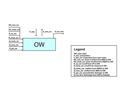
Figure 13 Schematic overview of Open Water (OW) in Urbanwb

2.8.1 Assumptions

All runoff from UP in a time step flows to OW in that same time step.
All sewer overflow into the street from SWDS and MSS in a time step flows directly to OW in that same time step.
A target OW level is defined as a level below the surface level. This is the lower limit of the OW level. For instance, the target OW level is set 1.5 m-SL, then the computed OW level x can only be higher than this level (x ≤ 1.5). Above this level (x < 1.5), discharge from OW to outside water starts. The outside water is not part of the model, and discharge from OW to outside is only limited by a predefined pumping capacity. Note, this pumping capacity can be applied as the discharge capacity in the Storage-Discharge-Frequency (SDF) curves, where the storages are calculation results of the Urbanwb.

2.8.2 Calculation order

Determine total runoff from UP to OW for the current time step.
Determine drainage from GW to OW for the current time step.
Determine total outflow from SWDS and MSS to OW and the total sewer overflow into the street from SWDS and MSS to OW for the current time step.
Determine inflow from measure (if applicable) to OW for the current time step.
Determine discharge from OW to outside water for the current time step.
Determine OW level at the end of the current time step.

2.8.3 Code and input arguments

class urbanwb.openwater.OpenWater(ow_no_meas_area, q_ow_out_cap, ow_level, **kwargs) [source]

Bases: _object

Creates an instance of OpenWater class with given initial states and properties, iterates sol() function to compute states and fluxes of Open Water at each time step.

Parameters:

ow_no_meas_area (float) – area of Open Water without measure [m^2]
q_ow_out_cap (float) – discharge capacity from Open Water (internal) to outside water (external) [mm/d]
ow_level (float) – predefined target Open Water level, also the initial Open Water level (at t=0) [m-SL]

sol(p_atm, e_pot_ow, r_up_ow, d_gw_ow, q_swds_ow, q_mss_ow, so_swds_ow, so_mss_ow, meas_ow, up_no_meas_area, gw_no_meas_area, swds_no_meas_area, mss_no_meas_area, tot_meas_area, tot_area, delta_t=0.041666666666666664) [source]

Calculates states and fluxes on Open Water during current time step.

Parameters:

p_atm (float) – rainfall during current time step [mm]
e_pot_ow (float) – potential Open Water evaporation during current time step [mm]
r_up_ow (float) – runoff from Unpaved to Open Water during current time step [mm]
d_gw_ow (float) – drainage from groundwater to Open Water during current time step [mm]
q_swds_ow (float) – Outflow from storm water drainage system (SWDS) to Open Water during current time step [mm]
q_mss_ow (float) – Outflow from combined sewer system (MSS) to Open Water during current time step [mm]
so_swds_ow (float) – Sewer overflow of storm water drainage system (SWDS) during current time step [mm]
so_mss_ow (float) – Sewer overflow of combined sewer system (MSS) during current time step [mm]
meas_ow (float) – inflow from measure (if applicable) to Open Water during current time step [mm]
up_no_meas_area (float) – area of Unpaved without measure [m^2]
gw_no_meas_area (float) – area of groundwater without measure [m^2]
swds_no_meas_area (float) – area of storm water drainage system (SWDS) without measure [m^2]
mss_no_meas_area (float) – area of combined sewer system (MSS) without measure [m^2]
tot_meas_area (float) – total area of measure [m^2]
tot_area (float) – total area of study area [m^2]
delta_t (float) – length of time step [d]

Returns: A dictionary of computed states and fluxes of Open Water during current time step:

prec_ow – Direct rainfall on Open Water during current time step [mm]
e_atm_ow – Evaporation from Open Water during current time step [mm]
sum_r_ow – Total runoff from Unpaved to Open Water during current time step [mm]
sum_d_ow – Drainage from groundwater to Open Water during current time step [mm]
sum_q_ow – Total outflow from sewer systems to Open Water during current time step [mm]
sum_so_ow – Total sewer overflow from sewer systems to Open Water during current time step [mm]
r_meas_ow – Inflow from measure (if applicable) to Open Water during current time step [mm]
q_ow_out – Discharge from Open Water to outside water during current time step [mm]

Return type: (dictionary)

2.9 Measure

Urban flooding is usually attributed to three types: pluvial flooding, fluvial flooding and coastal flooding. Pluvial flooding occurs when an extremely heavy rainfall saturates the storage capacity of the water system and excess water cannot be absorbed. Fluvial flooding occurs when rivers burst their bank as a result of sustained or intense rainfall. Coastal flooding occurs in coastal area as a result of extreme tidal conditions like storm surges. Unlike other types of flooding, pluvial flooding is a direct, quick and localized consequence of rainfall, and it is a predominantly urban phenomenon as it is in urban area where the effects are most pronounced and damaging (Susana). The Urbanwb model simulates only the pluvial flooding in urban water systems through two indicators, sewer overflow into the street and storage height above the target open water level. Climate change is predicted to increase the intensity and frequency of extreme rainfall events. Together with further urbanization and rapid growing population, this may result in increased urban pluvial flood risks. To effectively adapt to increasing flood risks, a combination of intervention strategies is required, including structural infrastructure, nature-based solutions, early warning system, risk financing instrument, etc. The Urbanwb model is capable of modelling all kinds of physical adaptation measures. Physical measures can be categorized into artificial structural infrastructure and nature-based solutions. Structural infrastructure refers to grey infrastructure are considered to be engineering projects that use concrete and steel, while nature-based solutions refer to blue-green infrastructure that depend on water, plants and ecosystem services. Blue-green infrastructure is the strategic use of networks of natural lands, working landscapes, and other open spaces to conserve ecosystem values and functions and provide associated benefits to human populations (Benedict & McMahon, 2006). Blue-green infrastructure is generally decentralized. Water is captured and treated where it falls, rather than being transported to a treatment facility. Blue-green infrastructure terminology can also be used in the context of low impact development (LID). Grey infrastructure refers to the human-engineered infrastructure for water resources such as water and wastewater treatment plants, pipelines, and reservoirs. Grey infrastructure typically refers to components of a centralized approach to water management. Examples of grey infrastructure are canals, levees, ditches, raised curbs, underground off-line tanks, etc. Examples of blue-green infrastructure are rainwater harvesting, water squares, urban wetlands, green roofs, bioswales, etc. A module named Measure is creatively developed in the Urbanwb model to model the physical urban adaptation measures. With the ingenious setup of this module, underlying mechanisms of these physical measures are simulated and incorporated into the dynamics of the entire modelling of water system. The next sections provide detailed descriptions on the structure of the Measure module.

Measures mitigate urban flooding by means of creating extra storage, encouraging evapotranspiration, facilitating infiltration, increasing drainage and the combination of these interventions. Consequently, despite many types/terms of urban adaptation measures, they can be categorized and modelled under certain framework with specific settings. The underlying idea and fundamental principle of this Measure module is to provide a general adaptive framework that represents the measures’ physical dimensions and that mimics the measures’ predominant functionality.

Measures in the Urbanwb model can be defined in a 1-layer, 2-layer or 3-layer structure (Figure 14 ).

Figure 14 Layer principle of measures in Urbanwb

1-layer structures contain only an interception layer (layer no. 1), which can represent the type of measures that creates storage and allows evaporation. A typical example of a 1-layer measure is a blue roof.

2-layer structures consist of 2 layers, an interception layer (layer no. 1) and a bottom storage layer (layer no.3). The bottom storage layer is the most sophisticated part of the measure module. In the bottom storage layer, evapotranspiration, percolation to groundwater and controlled runoff (to anywhere) can be defined by the user. Controlled runoff means the runoff volume that is first stored in the measure is discharged in a controlled way. Basically, controlled runoff implies either “continuously delayed released” to the urban water system or “instantaneously released at a much later time”, when the urban water system is able to handle this runoff again, most likely by means of real time control systems. Urban water system is referring to the entire water system, hence incorporating all elements described in the sections above. In the current Urbanwb model real time control is not incorporated and is simulated by a small constant discharge over a large number of time steps to one of the subsystems SWDS, GW, OW. Continuous slow release is defined as a dynamically-computed flux that dependents on a head difference and a flow resistance. Examples of 2-layer measures are rain barrel, wet pond, infiltration box, etc.

3-layer structures consist of 3 layers, an interception layer (layer no. 1), a top storage layer (layer no. 2) and a bottom storage layer (layer no.3). Extra, compared to the 2-layer measures is the top storage layer. This layer is especially added to model measures like green roofs and bioswales. These measures have a growing medium that encourages evapotranspiration and a drainage layer beneath the growing medium that drains excessive water to the sewer system. Some examples are provided in next paragraph to inspire the user how to conceptualize a measure into this Measure module.

The setup of the measures involves expert judgement: “the model is only as good as the modeler”.

Below some examples of how to conceptualize measures are provided:

Blue roof
Blue roofs (without drainage) create extra water storage on buildings from where water can evaporate. A blue roof can be considered as a storage installation. In the Urbanwb model, it can be simulated with the basic model or with the Measure module. Simulating a blue roof with the basic model can be done by increasing the PR interception capacity. However, then interception capacity of the entire PR area increases. To simulate that in only part of the PR area blue roofs are applied, the Measure module can be used. A blue roof can be conceptualized as a 1-layer structure of which an interception layer with certain storage capacity is defined from where only evaporation is possible. Exceedance of the storage capacity results in overflow. Overflow from a blue roof is considered to be uncontrolled runoff and will be drained to the SWDS.
Wet pond:
Figure 15 shows the schematic view of how wet pond is conceptualized. An artificial wet pond can be seen as a 2-layer structure, of which the interception layer is a pseudo layer that has no storage capacity and infinite infiltration capacity, allowing all water (precipitation and inflow runoff from contributing area) to flow directly into the bottom storage layer. A wet pond usually has a sealed concrete bottom to prevent it from falling dry thus percolation is defined not possible. The wet pond has a certain threshold (drainage level) above which the excess water is slowly drained. This runoff is called controlled runoff. The higher the water level in the pond above this threshold, the faster it drains. In addition, a drainage resistance has to be defined by the user to determine how fast it drains. Evaporation from the pool is possible and is limited by Penman evaporation. In case of very extreme rainfall events, incoming runoff may completely fill the storage capacity of wet pond, hence overflow from the wet pond occurs. Unlike controlled runoff from bottom storage layer, this overflow is an uncontrolled runoff, and will be drained eventually to SWDS.

Figure 15 Conceptualization of a wet pond. Source left figure: [LID].

Bioswale and green roof
Figure 16 shows the schematic view of how bioswale is conceptualized. A bioswale is an infiltration installation. An bioswale can be thought as a 3-layer structure, of which the surface vegetated soil is the interception layer that provides limited storage capacity and facilitates infiltration to the growing medium. The growing medium is the top storage layer where plant transpiration and soil evaporation occur. After evapotranspiration, excessive water infiltrates into the bottom drainage layer. Below the growing medium is the gravel drainage layer encouraging water percolating into the groundwater reservoir. Here the percolation flux can be modelled either as percolation to groundwater limited by saturated permeability of soil, or as a controlled runoff to groundwater dependent on predefined drainage level and resistance to mimic the water jamming. Evaporation from the bottom drainage layer is possible when potential evapotranspiration rate exceeds the transpiration from growing medium (top storage layer), to simulate that the plant roots can uptake water from drainage layer for further transpiration. Overflow from the bottom drainage layer and surface overflow from interception layer together form the uncontrolled runoff, which will be drained to the SWDS. Similar to a bioswale, a green roof is also modelled as a 3-layer structure. However, there are two major differences: 1. A green roof is installed on the building roof, thus controlled runoff directs to the SWDS instead of to GW; 2. The calculation formula for green roofs is specifically modified to make sure no surface submergence from green roof is possible because a normally functioning green roof should have no water logging on the surface.

Figure 16 Conceptualization of a bioswale. Source left figure: [LID].

2.9.1 Assumptions

A measure can be defined as 3-layer. Even though the area of each layer of measure can be defined different, it is not recommended to do so because it has not been fully tested yet.
The measure inflow area does not necessarily come from one source. For instance, if a measure is defined in the OP area, it is possible to define the measure inflow area not only in the OP area but also in the PR and the CP area. However, these possibilities have not been fully developed and tested yet. It’s users’ responsibility to pay attention to the boundary conditions of the model.
Not all measures can be implemented with Measure module or implemented with the Urbanwb model. The user should understand the correct way of using this Urbanwb model and should be careful with the limitations of this model.

2.9.2 Calculation order

Determine the rainfall on the measure for the current time step.
Determine the runoff from the measure inflow area to the measure for the current time step.
Determine the initial interception storage of measure. Initial interception water budge includes interception storage at the end of previous time step + rainfall + runoff from measure inflow area in case runoff is defined to flow to interception layer.
Determine the evaporation from the interception layer of the measure, limited by Penman evaporation.
Determine the downward infiltration from the interception layer. Downward infiltration from the interception layer is only possible when the measure structures contain at least 2 layers.
Note: Downward infiltration calculation for a green roof is separately defined.
Determine the surface overflow from the interception layer of the measure.
Determine the final interception storage on the interception layer of the measure.
Determine initial storage in top storage layer of measure. When measure structure contains only 2 layers. This storage is zeros (when 2 layer — no top storage layer is involved, all the variable related to top storage layer will be zero.) When 3 layer, initial storage in top storage layer of measure is storage at previous time step + downward infiltration from interception layer.
Determine transpiration from top storage layer of measure, limited by water availability and Penman evaporation multiplied with a predefined reduction factor.
Determine the percolation from the top storage layer of the measure to the bottom storage layer of the measure.
Note: This variable is separately defined for green roof type measures.
Determine the final storage in the top storage layer of the measure, limited by the predefined storage capacity of the top storage layer of the measure.
Determine the initial storage in the bottom storage layer of the measure.
Determine the evapotranspiration from the bottom storage layer of the measure. Transpiration from the bottom storage layer can only occur when defined possible and when the transpiration capacity exceeds the transpiration from the top storage layer in case of 3 layers.
Determine the percolation from the bottom storage layer of the measure to the groundwater. Specify whether this percolation is limited by the groundwater level or not. If not, the limitation will only be the saturated permeability. It is recommended to specify percolation being not limited by the groundwater level.
Determine the controlled runoff from the bottom storage level of the measure. The controlled runoff can be modelled as either a constant flux or as a dynamically-computed flux that depends on a user defined drainage level and resistance.
Determine the final storage of the bottom storage layer of the measure.
Determine the overflow from the bottom storage layer of the measure if the bottom layer is completely filled.
Determine the outflow from the measure to OW, UZ, GW, SWDS, MSS, Out

2.9.3 Code and input arguments

class urbanwb.measure.Measure(tot_meas_area, runoff_to_stor_layer, intstor_meas_t0, EV_evaporation, num_stor_lvl, infilcap_int_meas, storcap_top_meas, storcap_btm_meas, stor_top_meas_t0, stor_btm_meas_t0, storcap_int_meas, top_meas_area, ET_transpiration, evaporation_factor_meas, IN_infiltration, infilcap_top_meas, btm_meas_area, btm_meas_transpiration, connection_to_gw, limited_by_gwl, k_sat_uz, btm_level_meas, btm_discharge_type, runoffcap_btm_meas, dischlvl_btm_meas, c_btm_meas, surf_runoff_meas_OW, ctrl_runoff_meas_OW, overflow_meas_OW, surf_runoff_meas_UZ, ctrl_runoff_meas_UZ, overflow_meas_UZ, surf_runoff_meas_GW, ctrl_runoff_meas_GW, overflow_meas_GW, surf_runoff_meas_SWDS, ctrl_runoff_meas_SWDS, overflow_meas_SWDS, surf_runoff_meas_MSS, ctrl_runoff_meas_MSS, overflow_meas_MSS, surf_runoff_meas_Out, ctrl_runoff_meas_Out, overflow_meas_Out, greenroof_type_measure, **kwargs) [source]

Bases: _object

Creates an instance of Measure class with given initial states and properties, iterates sol() function to compute states and fluxes of measure at each time step.

Parameters:

tot_meas_area (float) – total area of measure [m^2]
num_stor_lvl (int) – predefined number of storage layers [1, 2 or 3]
runoff_to_stor_layer (int) – predefined selection at which measure layer runoff from other area is stored, inflow runoff can only take place at interception layer (1) or at bottom storage layer (3) [1 or 3]
Active processes (#) –
EV_evaporation (int) – predefined selection if evaporation from measure interception layer is possible (1) or not (0) [0 or 1]
ET_transpiration (int) – predefined selection if evapotranspiration from measure is possible (1) or not (0) [0 or 1]
IN_infiltration (int) – predefined selection if infiltration from measure is possible (1) or not (0) [0 or 1]
SD_delay (int) – predefined selection if slow drainage from measure is possible (1) or not (0) [0 or 1]
FD_pumping (int) – predefined selection if fast drainage from measure is possible (1) or not (0) [0 or 1]
RTC_realtime (#) – predefined selection if real- me-control release from measure is possible (1) or not (0) [0 or 1]
Interception layer (#) –
storcap_int_meas (float) – predefined storage capacity of interception layer of measure [mm]
infilcap_int_meas (float) – predefined infiltration capacity of interception layer of measure [mm/d]
stor_int_meas_t0 (float) – initial storage in interception layer of measure (at t=0) [mm]
Top storage layer (#) –
top_meas_area (float) – predefined area of top storage layer of measure [m^2]
storcap_top_meas (float) – predefined storage capacity of top storage layer of measure [mm]
infilcap_top_meas (float) – predefined infiltration capacity of top storage layer of measure [mm/d]
stor_top_meas_t0 (float) – initial storage in top storage layer of measure (at t=0) [mm]
Bottom storage layer (#) –
btm_meas_area (float) – predefined area of bottom storage layer of measure [m^2]
storcap_btm_meas (float) – predefined storage capacity of bottom storage layer of measure [mm]
connection_to_gw (int) – predefined percolation (connection) from measure bottom storage layer to groundwater is possible (1) or not (0) [0 or 1]
limited_by_gwl (int) – predefined limitation of percolation from measure to groundwater if groundwater level is below measure bottom level, limited (1) or unlimited (0) [0 or 1]
btm_level_meas (float) – predefined bottom level of measure [m-SL]
btm_meas_transpiration (int) – predefined selection if transpiration from bottom storage layer of measure is possible (1) or not (0) [0 or 1]
btm_discharge_type (int) – predefined discharge type from bottom storage layer of measure [0:flux or 1:level]
runoffcap_btm_meas (float) – predefined runoff capacity from bottom storage layer of measure [mm/d]
dischlvl_btm_meas (float) – predefined discharge level from bottom storage layer of measure [mm]
c_btm_meas (float) – predefined hydraulic resistance for level induced discharge from bottom storage layer of measure [d]
k_sat_uz (float) – saturation permeability of soil [mm/d]
evaporation_factor_meas (float) – predefined evaporation factor of measure [-]
stor_btm_meas_t0 (float) – initial storage in bottom storage layer of measure (at t=0) [mm]
Runoff from measure flows to (#) –
surf_runoff_meas_OW (int) – predefined definition of surface runoff from measure storage 1 (interception level) to Open Water (0 = no, 1 = yes)
ctrl_runoff_meas_OW (int) – predefined definition of controlled runoff from measure storage 3 (bottom level) to Open Water (0 = no, 1 = yes)
overflow_meas_OW (int) – predefined definition of overflow from measure storage 3 (bottom level) to Open Water (0 = no, 1 = yes)
surf_runoff_meas_UZ (int) – predefined definition of surface runoff from measure storage 1 (interception level) to Unsaturated Zone (0 = no, 1 = yes)
ctrl_runoff_meas_UZ (int) – predefined definition of controlled runoff from measure to Unsaturated Zone (0 = no, 1 = yes)
overflow_meas_UZ (int) – predefined definition of overflow from measure to Unsaturated Zone (0 = no, 1 = yes)
surf_runoff_meas_GW (int) – predefined definition of surface runoff from measure to groundwater (0 = no, 1 = yes)
ctrl_runoff_meas_GW (int) – predefined definition of controlled runoff from measure to groundwater (0 = no, 1 = yes)
overflow_meas_GW (int) – predefined definition of overflow from measure to groundwater (0 = no, 1 = yes)
surf_runoff_meas_SWDS (int) – predefined definition of surface runoff from measure to storm water drainage system (0 = no, 1 = yes)
ctrl_runoff_meas_SWDS (int) – predefined definition of controlled runoff from measure to storm water drainage system (0 = no, 1 = yes)
overflow_meas_SWDS (int) – predefined definition of overflow from measure to storm water drainage system (0 = no, 1 = yes)
surf_runoff_meas_MSS (int) – predefined definition of surface runoff from measure to mixed sewer system (0 = no, 1 = yes)
ctrl_runoff_meas_MSS (int) – predefined definition of controlled runoff from measure to mixed sewer system (0 = no, 1 = yes)
overflow_meas_MSS (int) – predefined definition of overflow from measure to mixed sewer system (0 = no, 1 = yes)
surf_runoff_meas_Out (int) – predefined definition of surface runoff from measure to outside water (0 = no, 1 = yes)
ctrl_runoff_meas_Out (int) – predefined definition of controlled runoff from measure to outside water (0 = no, 1 = yes)
overflow_meas_Out (int) – predefined definition of overflow from measure to outside water (0 = no, 1 = yes)

sol(p_atm, e_pot_ow, r_pr_meas, r_cp_meas, r_op_meas, r_up_meas, pr_no_meas_area, cp_no_meas_area, op_no_meas_area, up_no_meas_area, gw_no_meas_area, gwl_prevt, delta_t) [source]

Calculates states and fluxes in measure during current time step.

Parameters:

p_atm (float) – rainfall during current time step [mm]
e_pot_ow (float) – potential Open Water evaporation during current time step [mm]
r_pr_meas (float) – runoff from Paved Roof to measure during current time step [mm]
r_cp_meas (float) – runoff from Closed Paved to measure during current time step [mm]
r_op_meas (float) – runoff from Open Paved to measure during current time step [mm]
r_up_meas (float) – runoff from Unpaved to measure during current time step [mm]
pr_no_meas_area (float) – area of Paved Roof without measure [m^2]
cp_no_meas_area (float) – area of closed pave without measure [m^2]
op_no_meas_area (float) – area of Open Paved without measure [m^2]
up_no_meas_area (float) – area of Unpaved without measure [m^2]
gw_no_meas_area (float) – area of groundwater without measure [m^2]
gwl_prevt (float) – groundwater level at previous time step [m-SL]
delta_t (float) – length of time step [d]

Returns: A dictionary of computed states and fluxes of measure during current time step:

prec_meas – Direct rainfall on measure during current time step [mm]
sum_r_meas – Total runoff from Paved Roof, Closed Paved, Open Paved, Unpaved to measure during current time step [mm]
int_meas – Interception storage on interception layer of measure after rainfall at the beginning of current time step [mm]
e_atm_meas – Evaporation form interception layer of measure during current time step [mm]
interc_down_meas – Downward flow from interception layer of measure during current time step [mm]
surf_runoff_meas – Surface runoff from interception layer of measure during current time step [mm]
intstor_meas – Remaining interception storage on interception layer of measure during current time step [mm]
ini_stor_top_meas – Storage in top storage layer of measure at the beginning of current time step [mm]
t_atm_top_meas – Transpiration from top storage layer of measure during current time step [mm]
perc_top_meas – Percolation from top layer of measure at the current time step [mm]
fin_stor_top_meas – top layer storage at the end of current time step [mm]
ini_stor_btm_meas – bottom layer storage at the beginning of current time step [mm]
t_atm_btm_meas – transpiration from bottom layer of measure at the current time step [mm]
p_gw_btm_meas – percolation from bottom layer of measure to groundwater during current time step [mm]
runoff_btm_meas – runoff from the bottom layer of the measure during current time step [mm]
fin_stor_btm_meas – bottom storage at the end of the current time step [mm]
overflow_btm_meas – bottom storage overflow during current time step [mm]
q_meas_ow – Measure outflow to Open Water during current time step [mm]
q_meas_uz – Measure outflow to Unsaturated Zone during current time step [mm]
q_meas_gw – Measure outflow to groundwater during current time step [mm]
q_meas_swds – Measure outflow to storm water drainage system during current time step [mm]
q_meas_mss – Measure outflow to mixed sewer system during current time step [mm]
q_meas_out – Measure outflow to outside water during current time step [mm]

Return type: (dictionary)

3 FAQ

What are area with measure, area without measure and measure inflow area?

Figure 17 Illustration of measure inflow area

All individual areal components of the simulation model, PR, OP, etc., mentioned in the documentation, basically are all areas without applied measure. Figure 17 shows an example of applying a measure on OP. If the (green) measure area is 2 m2, and the total OP area is 10 m2, the (blue + grey) area of OP without measure is 10 – 2 = 8 m2.
The measure inflow area (green + blue) should always be larger than (or equal to) the measure area (green) and limited by the total paved area (green + blue + grey). The total measure inflow area can be larger than the total OP area in the example, when also part of the PR and / or the CP area runoff is diverted to the measure inflow area in OP.

4 References for parameter estimations

Penman, H. L. (1948). Natural evaporation from Open Water, bare soil and grass. Proceedings of the Royal Society of London. Series A. Mathematical and Physical Sciences, 193(1032), 120145.
Monteith, J. L. (1965, July). Evaporation and environment. In Symp. Soc. Exp. Biol (Vol. 19, No. 205-23, p. 4).
Feddes, R.A., Kowalik, P.J., Zaradny, H., (1978). Simulation of filed water use and crop yield. Simulation Monographs. Pudoc, Wageningen, 189pp
DE JONG VAN LIER, Q., et al (2008). Macroscopic root water uptake distribution using a matric flux potential approach. Vadose Zone Journal, 2008, 7.3: 1065-1078.
Allen, R.G., Pereira, L.S., Raes, D., and Smith, M. 1998. Crop evapotranspiration: Guidelines for computing crop water requirements. FAO Irrigation and Drainage Paper No. 56, United Nations, FAO, Rome, Italy.
STOWA, 2009 rapport 11. VERBETERING BEPALING ACTUELE VERDAMPING VOOR HET STRATEGISCH WATERBEHEER. isbn 978.90.5773.428.1
Makkink, G. F. (1957). Testing the Penman formula by means of lysimeters. Journal of the Institution of Water Engineers, 11, 277-288.
Susana, Urban pluvial flooding and climate change: London (UK), Rafina (Greece) and Coimbra (Portugal).
Benedict, M. A., & McMahon, E. T. (2006). Green infrastructure. Island, Washington, DC.
LID, Low impact development — a design manual for urban areas.

5 Running the model

5.1 Overview

The script model can be run from windows command prompt or with _run.bat file. The latter choice is highly recommended.

For the time being, the most commonly used function is savecsv, batch-run-sdf and batch-run-measure

The _{running_sample} folder in the Urbanwb package includes the sample of running the model for both basic model and model with measure.

Two sorts of input are necessary to start the Urbanwb model:

Dynamic_input: The forcing — Hourly time series of Precipitation, potential Open Water evaporation and potential reference crop evapotranspiration. The user is responsible for data preprocessing — clean data, fill vacancy, remove unrealistic data and make sure the data is in float type. Make sure the column name is the same because script use the column name to index which data is precipitation and evaporation.

Static_input: All the static input parameters are stored in the configuration file suffixed with _.ini. Currently, two configuration files are indispensable for every function to use — one is neighbourhood configure file, the other is measure configuration file. If no measure is included in the modelling, please specify _{measure_appled=false} in measure configuration file. Though the script will automatically do some checks after reading the configuration file to make it fool proof, for example it will update the measure-related area with zero if no measure is applied even if it is not zero due to user’s carelessness, it is highly recommended that user carefully deal with the configuration input. Besides, user should modify the parameters according to the local context of his area of interest and expected setups. Be aware of not changing the parameter name, otherwise the model goes wrong. The descriptions of the parameter are in the configuration file, documentation and script docstrings for user’s cross check.

5.2 Input time series and parameters

5.2.1 Time series (Dynamic input)

The forcing of Urbanwb model is the time series of:

precipitation (only rainfall considered)
potential Open Water evaporation (i.e. Penman evaporation – Penman, 1948)
potential reference crop evapotranspiration (i.e. Penman-Monteith evaporation – Montheith, 1965 or Makkink evaporation – Makkink, 1957)

Note:

Sometimes, Penman evaporation is not directly available since it is not straightly measured, while (class-A) pan evaporation data is easier to find. Pan evaporation Usually, pan evaporation is multiplied a correlation factor 0.77 to convert to Penman evaporation (Linacre, 1994). The model assumes potential Open Water evaporation actual interception evaporation on paved surface

Even though Forcing: Hourly time series of precipitation (actually only rainfall) [mm] and potential evaporation of Open Water [mm]. (for grass, it is approximately 0.8982 * Penman evaporation – Droogers, 2009) Length should better be most recent 30 years. Atmosphere is the most crucial exchange to the model. 1. Format: CSV format is preferred with corresponding column names. Make sure the data has no vacancy or unrealistic data. Make sure the data is in float type. 2. Note: Sometimes hourly potential Open Water evaporation is not findable, and it may be easier to get access to data like class-A pan evaporation time series. However, pan evaporation cannot be used as input directly. Conversion from pan evaporation to Penman Open Water evaporation should be done before running the model. Sometimes it is possible that only daily evaporation time series is available or even daily evaporation time series is not available, then assumptions and simplifications will be made on evaporation interpolation. For instance, in Area H, we only have annual potential evaporation data. First, we will divide this value by 365 to get the average daily evaporation. Then, interpolate by daily dynamics as assumed.

5.2.2 Parameters (Static input)

Land use at or above surface level are divided into 5 components, namely Paved Roofs (buildings), Closed Paved (roads, etc.), Open Paved (pavements, parkings, etc.), Unpaved (grass land, etc.) and Open Water (ditches, canals, ponds, etc.). The fractions of the five land use types should sum up to 100%. And we need total area of the study area in [m2] Besides, for paved areas (PR, CP, OP), we also can define three additional types of fractions:

disconnected fraction of three paved areas: “Part disconnected from sewer”: This disconnect fraction means how much percentage of the paved area (say Paved Roofs) is disconnected from the sewer system. If this fraction is 5%, then it means 5% of the Paved Roofs (PR) is disconnected to sewer system. Consequently, 5% of the runoff from the Paved Roofs (PR) will not end in the sewer system but will presumably flow to Unpaved area.
part of building above groundwater (GW): “part of buildings above GW”: This fraction means, in terms of Paved Roofs only, how much percentage of Paved Roofs (PR) has its bottom of foundation above the phreatic table. As we know, the relationship between the bottom level of building foundation and variation of groundwater level is essential to building stability, but this safety concern is not the model concern. What this fraction really matters in the model is the total area size of the (shallow) groundwater (GW).
part of Open Water above groundwater (GW): “Part of OW above GW”: This fraction is more or less similar to part of building above groundwater (GW). It affects the calculation of size of groundwater area. Say we have 300m2 Open Water. If this fraction is zero, then groundwater will not contain any m2 of this 300m2. If this fraction is 100%, then groundwater will contain this extra 300m2 as all Open Water is above the groundwater. To sum up, type 2 and type 3 fractions influence the total area of (shallow) groundwater (GW). Area is important since all the storage and fluxes in the model are calculated in depth [mm], so the conversion from one component to another component is dependent on the area ratio of two components. That is the reason why two additional fractions (type 2 and type 3) are defined to decide the groundwater area more precisely.

Runoff from paved surface to sewer system only occurs when surface interception storage capacity can no longer handle excessive rainfall. “Storm Water Drainage System”: Part of urban area with storm water drainage system. “Mixed Sewer System”: Part of urban area with mixed sewer system (i.e. combined sewer system). These two fractions should sum up to 100%.

Design standard / Design rainfall of sewer system. This part may be a bit confusing, please don’t get puzzled by the nota on used i. Circle 3.b is discharge capacity of SWDS to Open Water, discharge capacity of MSS to Open Water (wet flow condition), discharge capacity of MSS to waste water treatment plant (dry flow condition). These three discharge capacities in circle 3.b are used in the model. Circle 3.a is design rainfall. Parameters in Circle 3.a are not directly used in the model. They are actually used to calculated Circle 3.b parameters if there is no direct information on design discharge capacity of sewer system. In the Netherlands, say if there is no direct information on discharge capacity of SWDS to Open Water (actually there is and it is around 21mm/hr to 30mm/hr), then we can do below calculations: “t = 2 rainfall” (in Fig 2): Design rainfall intensity of sewer system. In the Netherlands, the sewer overflow on the street is designed to occur once every two years. Hence t = 2 year is chosen as the design rainfall return period. Its corresponding rainfall intensity is 58.7 mm/hr by rainfall statistics. Consequently, for SWDS, the predefined discharge capacity of the SWDS is then calculated as 58.7(rainfall intensity of t=2) - 1.6 (interception on paved area) – 2 (storage in SWDS) = 55.1 mm/hr. This 55.1mm/hr is the discharge capacity of SWDS to Open Water above which sewer water will overflow onto the street. Similar to SWDS, discharge capacity of MSS to Open Water is calculated as 48.1mm/hr above which sewer overflow from MSS onto street will occur. “t = 1/6 rainfall” (in Fig 2): Design rainfall intensity of combined sewer overflow. In the Netherlands, the combined sewer overflow onto the Open Water is designed to occur six to seven times a year. Hence t= 1/6 is chosen as the design rainfall return period of combined sewer overflow. Its corresponding rainfall intensity is 27.9 mm/hr by statistics. Consequently, for MSS, the predefined discharge capacity of the MSS to waste water treatment plant (WWTP) is in fact the sewer discharge capacity above which sewer overflow to Open Water (CSO) will occur, and this discharge capacity is calculated as 27.9 – 1.6 = 26.3mm/hr.

5.3 Functions

5.3.1 save_to_csv

This function performs single run of the model. It can save all results or selected results in to an output csv file.

# save all results

# module name func name timeseries name neighbourhood measure outputfile

python -m urbanwb.main_with_measure save_to_csv timeseries.csv config1.ini config2.ini output.csv

# save selected results

# module name func name timeseries name neighbourhood measure outputfile variable to save save_all is False -> save selected

python -m urbanwb.main_with_measure save_to_csv timeseries.csv config1.ini config2.ini output.csv owl r_pr_swds theta_uz --save_all=False

5.3.2 batch_run_sdf

This function performs batch run on different pumping capacity to produce database which can be used to plot Storage-Discharge-Frequency (SDF) Curve

Running the model — urbanwb 0.1.0 documentation

# mean daily rainfall as baseline q, batch run [4,5]

# module name function ts.csv config1.ini config2.ini output.csv random number baseline q default

python -m urbanwb.main_with_measure batch_run_sdf ep_ts.csv ep_neighbourhood.ini ep_measure.ini ep2_results.csv --q_list=[4,5]

# 4 as baseline q, batch run [10,20]

# module name function ts.csv config1.ini config2.ini output.csv random number baseline q predefined

python -m urbanwb.main_with_measure batch_run_sdf ep_ts.csv ep_neighbourhood.ini ep_measure.ini ep2_results1.csv --q_list=[10,20] --baseline_q=4

# 3 as baseline q, batch run [min,max,steps] --- [4,8,3]

# module name function ts.csv config1.ini config2.ini output.csv [min,max,steps] baseline q:predefined AP: True to enable [min,max,steps]. if False, then q_list random numbers

python -m urbanwb.main_with_measure batch_run_sdf ep_ts.csv ep_neighbourhood.ini ep_measure.ini ep2_results2.csv --q_list=[4,8,3] --baseline_q=3 --arithmetic_progression=True

5.3.3 batch_run_meas

This function performs batch run on measure. First do batch run with different (pairs of) values, then do baseline run (no measure). In the end, save the runoff time series into a csv file.

It can vary one parameter with a list of values or vary two parameters at the same time.

# module function ts.csv config1.ini config2.ini output.csv var to change value to update var corresp var value for corresp var baseline runoff measure runoff to save

python -m urbanwb.main_with_measure batch_run_measure ep_ts.csv ep_neighbourhood.ini ep_measure.ini ep3_results.csv --varkey="storcap_btm_meas" --vararrlist1=[1050,1200] --correspvarkey=None -vararrlist2=None --baseline_variable="r_cp_swds" --variable_to_save="q_meas_swds"

python -m urbanwb.main_with_measure batch_run_measure ep_ts.csv ep_neighbourhood.ini ep_measure.ini ep3_results.csv --varkey="storcap_btm_meas" --vararrlist1=[1050,1200] --correspvarkey="runoffcap_btm_meas" --vararrlist2=[30,40] --baseline_variable="r_cp_swds" -riable_to_save="q_meas_swds"

python -m urbanwb.getconstants ep3_results.csv --num_year=30

5.4 References

DROOGERS, P. Verbetering bepaling actuele verdamping voor het strategisch waterbeheer. Definitiestudie. STOWA, 2009.
PENMAN, Howard Latimer. Natural evaporation from Open Water, bare soil and grass. Proc. R. Soc. Lond. A, 1948, 193.1032: 120-145.
MONTEITH, John L., et al. Evaporation and environment. In: Symp. Soc. Exp. Biol. 1965. p. 4.
LINACRE, Edward T. Estimating US Class A pan evaporation from few climate data. Water International, 1994, 19.1: 5-14.

Space shortcuts

Page tree

Urban Water balance model

1 General description

1.1 Introduction

1.2 Major components

1.3 General assumptions

2 Model components

2.1 Paved Roof

2.1.1 Assumptions

2.1.2 Calculation order

2.1.3 Code and input arguments

2.2 Closed Paved

2.2.1 Assumptions

2.2.2 Calculation order

2.2.3 Code and input arguments

2.3 Open Paved

2.3.1 Assumptions

2.3.2 Calculation order

2.3.3 Code and input arguments

2.4 Unpaved

2.4.1 Assumptions

2.4.2 Calculation order

2.4.3 Code and input arguments

2.5 Unsaturated Zone

2.5.1 Assumptions

2.5.2 Calculation order

2.5.3 Code and input arguments

2.6 Groundwater

2.6.1 Assumptions

2.6.2 Calculation order

2.6.3 Code and input arguments

2.7 Sewer system

2.7.1 Assumptions

2.7.2 Calculation order

2.7.3 Code and input arguments

2.8 Open Water

2.8.1 Assumptions

2.8.2 Calculation order

2.8.3 Code and input arguments

2.9 Measure

2.9.1 Assumptions

2.9.2 Calculation order

2.9.3 Code and input arguments

3 FAQ

4 References for parameter estimations

5 Running the model

5.1 Overview

5.2 Input time series and parameters

5.2.1 Time series (Dynamic input)

5.2.2 Parameters (Static input)

5.3 Functions

5.3.1 save_to_csv

5.3.2 batch_run_sdf

5.3.3 batch_run_meas

5.4 References