03 Display Groups

Introduction

A list of pre-configured displays can be configured in the Display groups. When available on the file system, the name of the XML file is for example: DisplayGroups 1.00 default.xml

The pre-configured displays are organised in a tree view in the time series display (see example in Figure 1). Each pre-configured display is identified by its name, and may include one or more subplots, each with one or more time series lines.

Figure 1 Example of time series display, showing two sub-plots and tree-view of pre-configured displays

Another option is to plot a longitudinal profile in the time series display (see figure 2). The main difference with the normal time series plot is, that on the X-axis the river chainage is plotted. With the control toolbar a specific time step can be selected.

Figure 2 Example of time series display, showing longitudinal profile.

The display groups are configured by first listing the names of the filters to be shown in the display (for example "Rain gauges", "Gauges" and "Fractions" in figure 3 below) under the displayGroup descriptor. The names of the subplots can then be added (e.g. "MacRitchie" and "Woodleigh" below). Each of the subplots is assigned a plotId which links to the definitions of the plots and the time series set to be used. For example in the Fractions displayGroup a stackPlot is defined with a max and min (this file is attached as an example). Please note that the colours, linestyle, precision etc are defined in the TimeSeriesDisplayConfig.

figure 3 - example of a configured displayGroup file (click to enlarge)

Figure 4 Root element of the display groups definition

displayGroups

Root element for each displayGroup. A display group forms one of the main nodes in the tree view and may contain multiple displays. Multiple display groups may be defined.

Attributes:

• description: Optional description
• plot: Plot complex type
• displayGroup: displayGroup complex type

plot

Defines the plots relating to the displayGroup

Elements:

• description: Description of plot
• legendFontSize: Font size of legend
• axis TitleFontSize: Title font size
• tickLableFontSize: Option to change tick label font size
• synchronizeParameterAxis: Since 2018.02. Option to synchronize the axis range of subplots displaying time series for the same parameter group. 
• subplot: Link to subplot complex type.

displayGroup

Defines the groups of plots to be viewed (i.e. the branches of the shortcuts in the display)

Attributes:

• description: Optional description
• display: Display complex type
• displayGroup: displayGroup which links to the plot id

subplot

Root element for each subplot. Multiple sub-plots may be defined per display.

Attributes:

• description
• axisScaleUnit: Unit used for rounding the min and max value of the axis. If scale unit = 1 then a range of -3.8 to 4.9 will be rounded to a range of -4 to 5
• lowerMarginPercentage:
• upperMarginPercentage:
• barMarginPercentage: Since 2018.02. Only applicable for subplots which contain bars, such as plots of <subPlotType> "horizontalColorCode" or bar charts. Percentage of the bar width by which the bar width will be reduced, to create space between the bars. Default value is the barMarginPercentage in the generalDisplayConfig of the TimeSeriesDisplayConfig.xml (which is 0 by default). Use the general option to set a barMarginPercentage to be applied to all plots containing bars. Use this config option to overrule the general barMarginPercentage for a specific subplot.
• inverted
• plotweight
• plotSeparatorWeight
• thresholdAxisScaling
• forecastConfidenceTimeSpan: TimeSpanComplexType
• line
• area: Fills the area between multiple time series.
• color: Overides colours specified in the timeseriesdiplay
• lineStyle: Line style of time series marker line. Enumeration of "solid", "none", "bar", "dashdot", "dashed", "dotted". When a suffix of ";thick" is given, 1 will be added to the linewidth found in the TimeSeriesDisplayConfig.xml. For example, if a linewidth of 2 is configured in the TimeSeriesDisplayConfig and for a subplot the linestyle is set to "solid;thick", the resulting linewidth will be 2 + 1 = 3.
• timeSeriesSet

subPlotType

By default the <subPlotType> is set to 'standard', which means the default plot type for the configured timeSeriesType will be used. Optionally, you can configure the following other subplot types.

stack

Time series of this subplot are plotted as stacked areas (if lineStyle is solid) or stacked bars (if lineStyle is bar).

colorMapBars

Time series of this subplot are plotted as stacked bars. Color of the bar matches the paint scale color associated with the bar value. Height of all bars is the same, and equals Y-axis  range / number of series in the plot.

horizontalColorCode

A horizontal bar is plotted for each time series. The color of the bars signify the value for that time series at the given time on the x-axis.

horizontalColorCode Example <plot id="HorizontalColorCodePumps"> <description>testing the horizontal color code plots</description> <subplot> <subPlotType>horizontalColorCode</subPlotType> <barMarginPercentage>30</barMarginPercentage> <classBreaks> <break lowerValue="0" color="green" label="off"/> <break lowerValue="1" color="goldenrod" label="1 pump"/> <break lowerValue="2" color="magenta" label="2 pumps"/> <break lowerValue="3" color="aquamarine" label="3 pumps"/> <break lowerValue="4" color="red"/> </classBreaks> <timeSeriesSet> <moduleInstanceId>Preprocess_Units_HTMS</moduleInstanceId> <valueType>scalar</valueType> <parameterId>PO_BFN</parameterId> <locationId>BFN Tower 1</locationId> <locationId>BFN Tower 2</locationId> <locationId>BFN Tower 3</locationId> <locationId>BFN Tower 4</locationId> <locationId>BFN Tower 5</locationId> <locationId>BFN Tower 6</locationId> <locationId>BFN Tower 7</locationId> <timeSeriesType>simulated forecasting</timeSeriesType> <timeStep unit="hour" multiplier="1"/> <readWriteMode>read only</readWriteMode> </timeSeriesSet> </subplot> </plot>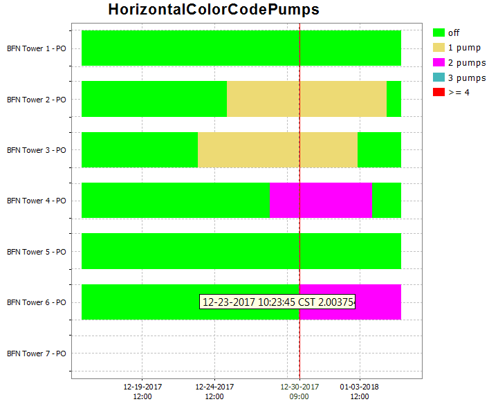

Vertical line fill

Use the <area> element in combination with a <lineStyle> to obtain vertical lines.

<subplot>
     <area>
        <lineStyle>solid</lineStyle>
        <lineWidth>10</lineWidth>
         <color>blue</color>
         <opaquenessPercentage>50</opaquenessPercentage>
           <timeSeriesSet>
                <moduleInstanceId>ImportMSW</moduleInstanceId>
                <valueType>scalar</valueType>
                <parameterId>Q.m</parameterId>
                <locationId>H-MS-LUIK</locationId>
                <locationId>H-MS-SINT</locationId>
                <timeSeriesType>external historical</timeSeriesType>
                <timeStep unit="hour"/>
                <relativeViewPeriod unit="day" start="-2" end="0"/>
                <readWriteMode>read only</readWriteMode>
           </timeSeriesSet>
        </area>
</subplot>

inverted

This tag can be used to invert the y-axis of a plot. Below a screenshot of an inverted graph. In the example the timeseries with parameter RAIM is inverted.

line

The tag line can be used to configure both single or dual y-axis. Enables the configuration of a custom colour. visibleInLegend and visibleInTable are optional, default setting is true. If visibleInLegend is set to false, the series will show up in the plot area, but not in the legend. If visibleInTable is set to false, the time series can still be sen on the plot, but the data will not show in the table.

Example:

<plot id="Test">
   <subplot>
      <line>
         <color>dark orange</color>
         <visibleInLegend>false</visibleInLegend>
         <visibleInTable>false</visibleInTable>
         <timeSeriesSet>
         <moduleInstanceId>Import</moduleInstanceId>
         <valueType>scalar</valueType>
         <parameterId>H.m</parameterId>
         <locationId>LocA</locationId>
         <timeSeriesType>external historical</timeSeriesType>
         <timeStep unit="hour"/>
         <relativeViewPeriod unit="hour" start="-12" end="12"/>
         <readWriteMode>editing visible to all future task runs</readWriteMode>
      </timeSeriesSet>
   </line>           
   </subplot>
</plot>

Dual y-axis plots

It is possible to have two y-axis visible in the same plot. This can be done by having multiple timeseries where some are assigned to the left y axis and some to the right y axis, or by having a timeseries on the left y axis with an associated rating curve on the right y axis. So every timeseries plot (also in reports) will have a mandatory left y axis to which a timeseries is associated and an optional right y axis to which a timeseries or rating curve is associated.

The display of threshold lines are supported for one y axis. But there can be threshold lines for either the left or the right y axis, but not both.

Multiple TimeSeries plots

To associate a timeseries to the left or right y axis use the <axis> element. This element is optional and leaving it out will associate it (default) to the left axis. Please note that at least one timeseries should be on the left axis (by either settings <axis>left</axis> or leaving the element out and using the default).

Below are two examples of a config and the resulting plot.

		<subplot>
			<plotWeight>1</plotWeight>
			<line>
				<color>blue</color>
				<axis>left</axis>
				<timeSeriesSet>
					<moduleInstanceId>ImportTelemetry</moduleInstanceId>
					<valueType>scalar</valueType>
					<parameterId>H.obs</parameterId>
					<locationId>Hydro1</locationId>
					<timeSeriesType>external historical</timeSeriesType>
					<timeStep unit="minute" multiplier="15"/>
					<relativeViewPeriod unit="hour" start="-36" end="36"/>
					<readWriteMode>editing visible to all future task runs</readWriteMode>
				</timeSeriesSet>
			</line>
			<line>
				<color>blue</color>
				<axis>left</axis>
				<timeSeriesSet>
					<moduleInstanceId>ImportTelemetry</moduleInstanceId>
					<valueType>scalar</valueType>
					<parameterId>H.rated</parameterId>
					<locationId>Hydro3</locationId>
					<timeSeriesType>external historical</timeSeriesType>
					<timeStep unit="minute" multiplier="15"/>
					<relativeViewPeriod unit="hour" start="-36" end="36"/>
					<readWriteMode>editing visible to all future task runs</readWriteMode>
				</timeSeriesSet>
			</line>
			<line>
				<color>red</color>
				<axis>right</axis>
				<timeSeriesSet>
					<moduleInstanceId>ImportTelemetry</moduleInstanceId>
					<valueType>scalar</valueType>
					<parameterId>Q.obs</parameterId>
					<locationId>Hydro2</locationId>
					<timeSeriesType>external historical</timeSeriesType>
					<timeStep unit="minute" multiplier="15"/>
					<relativeViewPeriod unit="hour" start="-36" end="36"/>
					<readWriteMode>editing visible to all future task runs</readWriteMode>
				</timeSeriesSet>
			</line>
			<line>
				<color>red</color>
				<axis>right</axis>
				<timeSeriesSet>
					<moduleInstanceId>ImportTelemetry</moduleInstanceId>
					<valueType>scalar</valueType>
					<parameterId>Q.rated</parameterId>
					<locationId>Hydro4</locationId>
					<timeSeriesType>external historical</timeSeriesType>
					<timeStep unit="minute" multiplier="15"/>
					<relativeViewPeriod unit="hour" start="-36" end="36"/>
					<readWriteMode>editing visible to all future task runs</readWriteMode>
				</timeSeriesSet>
			</line>
		</subplot>

		<subplot>
			<plotWeight>1</plotWeight>
			<line>
				<color>blue</color>
				<axis>right</axis>
				<timeSeriesSet>
					<moduleInstanceId>ImportTelemetry</moduleInstanceId>
					<valueType>scalar</valueType>
					<parameterId>H.obs</parameterId>
					<locationId>Hydro1</locationId>
					<timeSeriesType>external historical</timeSeriesType>
					<timeStep unit="minute" multiplier="15"/>
					<relativeViewPeriod unit="hour" start="-36" end="36"/>
					<readWriteMode>editing visible to all future task runs</readWriteMode>
				</timeSeriesSet>
			</line>
			<line>
				<color>red</color>
				<timeSeriesSet>
					<moduleInstanceId>ImportTelemetry</moduleInstanceId>
					<valueType>scalar</valueType>
					<parameterId>Q.obs</parameterId>
					<locationId>Hydro2</locationId>
					<timeSeriesType>external historical</timeSeriesType>
					<timeStep unit="minute" multiplier="15"/>
					<relativeViewPeriod unit="hour" start="-36" end="36"/>
					<readWriteMode>editing visible to all future task runs</readWriteMode>
				</timeSeriesSet>
			</line>
		</subplot>

Stage/discharge plots

When a discharge is displayed, it is possible to show the stage on the right axis. It is not possible to configure this rating on the left axis (and the timeseries on the right axis), since a plot has to have at least one timeseries on the left axis.

The right axis is then not a linear axis but the ticks on the right axis are calculated from the discharge ticks on the left axis.

It is also possible to display the stage and show the discharge on the right axis. The example below shows a display which plots several discharge time series.

The left axis is a linear axis with ticks for the discharge. The right axis is a non-linear axis.

The ticks on the right axis are calculated from the value of the discharge on the left axis by using a rating curve.

Below an configuration and resulting plot

<subplot>
			<line>
				<color>black</color>
				<lineStyle>none</lineStyle>
				<markerStyle>+</markerStyle>
				<markerSize>3</markerSize>
				<timeSeriesSet>
					<moduleInstanceId>ImportTelemetry</moduleInstanceId>
					<valueType>scalar</valueType>
					<parameterId>Q.rated</parameterId>
					<locationId>Hydro4</locationId>
					<timeSeriesType>external historical</timeSeriesType>
					<timeStep unit="minute" multiplier="15"/>
					<relativeViewPeriod unit="hour" start="-36" end="36"/>
					<readWriteMode>editing visible to all future task runs</readWriteMode>
				</timeSeriesSet>
			</line>
			<line>
				<color>black</color>
				<lineStyle>solid</lineStyle>
				<markerStyle>circle</markerStyle>
				<markerSize>6</markerSize>
				<axis>left</axis>
				<ratingAxis>
					<parameterGroupId>Water Level</parameterGroupId>
					<transformationType>dischargeStage</transformationType>
				</ratingAxis>
				<timeSeriesSet>
					<moduleInstanceId>ImportTelemetry</moduleInstanceId>
					<valueType>scalar</valueType>
					<parameterId>Q.obs</parameterId>
					<locationId>Hydro2</locationId>
					<timeSeriesType>external historical</timeSeriesType>
					<timeStep unit="minute" multiplier="15"/>
					<relativeViewPeriod unit="hour" start="-36" end="36"/>
					<readWriteMode>editing visible to all future task runs</readWriteMode>
				</timeSeriesSet>
			</line>
		</subplot>

descriptiveFunctions

Adding DescriptiveFunctions will result in an extra panel in the display, showing relevant descriptive information about the timeseries in view. More information on the descriptive functions available can be found onTimeSeriesDisplayConfiguration

VariableLineWidth

Options available when creating an variable line width type display

Attributes:

• markerColor: option to set marker color different from line color
• lineWidthScaleFactor: factor to increase or decrease the line width
• valueTimeSeriesSet: Time series for XY line plot
• lineWidthTimeSeriesSet: Time series for line width of the XY plot lines

Example

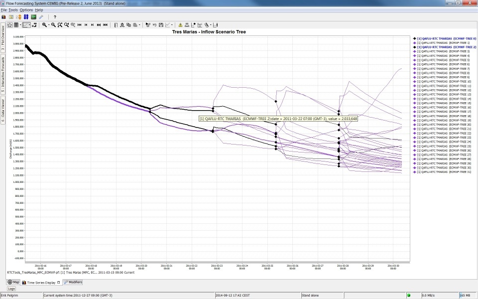
Below a screenshot of a variable line width plot for different ensemble members that have different line width's. In this case line width is an indication of the probability of the ensemble member. The sum of probability of all ensemble members at a time is one. Selecting separate ensemble members will mark them with the color black.

Single location displays can be used to easily create plots for individual locations. This can either be done for individual locations, or alternatively for a locationSet which will then produce a list of location with their corresponding plot.

Chainage location set

(Since 2016.02) By using a chainage location set in a time series set of a plot in the display groups, a longitudinal profile can be plot based on scalar time series for different locations

<displayGroups version="1.0" xmlns="http://www.wldelft.nl/fews" xmlns:xsi="http://www.w3.org/2001/XMLSchema-instance" xsi:schemaLocation="http://www.wldelft.nl/fews http://fews.wldelft.nl/schemas/version1.0/displayGroups.xsd">
	<plot id="Langsprofiel_Caspargouwse_Wetering">
		<subplot>
			<timeSeriesSet>
				<moduleInstanceId>WerkFilter</moduleInstanceId>
				<valueType>scalar</valueType>
				<parameterId>H.G.15</parameterId>
				<chainageLocationSetId>Langsprofiel_Caspargouwse_Wetering</chainageLocationSetId>
				<timeSeriesType>external historical</timeSeriesType>
				<timeStep unit="minute" multiplier="15"/>
				<relativeViewPeriod unit="day" start="-32" end="0"/>
				<readWriteMode>read only</readWriteMode>
			</timeSeriesSet>
		</subplot>
	</plot>
	<displayGroup name="LangsProfiel">
		<display name="Langsprofiel_Caspargouwse_Wetering">
			<locationSetId>Langsprofiel_Caspargouwse_Wetering</locationSetId>
			<plotId>Langsprofiel_Caspargouwse_Wetering</plotId>
		</display>
	</displayGroup>
</displayGroups>

Notice that it is not possible to combine a longitudinal plot in with a standard plot (having time on the X-axis). Furthermore, it is not possible to use it for relatedLocations, and also thresholds will not be shown.

Single Domain Axis Time Series (1D Spectra plots)

Time series with one domain axis are displayed as one xy chart per time step, like longitudinal profiles. A slider is used to navigate through time.

<timeSeriesSet>
	<moduleInstanceId>LMW_Import_spectrum</moduleInstanceId>
	<valueType>scalar</valueType>
	<parameterId>Wave.variancedensity.meting</parameterId>
	<domainParameterId>f</domainParameterId>
	<locationSetId>LMW_Czz10</locationSetId>
	<timeSeriesType>external historical</timeSeriesType>
	<timeStep unit="minute" multiplier="60"/>
	<relativeViewPeriod unit="day" start="-2" end="2"/>
	<readWriteMode>read only</readWriteMode>
</timeSeriesSet>

Dual Domain Axis Time Series (2D Polar Spectra plots)

When a second domain axis is available this will always be used as direction for a polor plot by the time series dialog. When second domain axis is not a directional parameter or the time series has more than two domain axes the time series can not be diplayed the time series dialog with the current functionality

<subplot>
	<classBreaks>
		<break symbolSize="10" color="000080" lowerValue="0"/>
		<break symbolSize="10" color="0000A8" lowerValue="0.0005"/>
		<break symbolSize="10" color="0000E6" lowerValue="0.001"/>
		<break symbolSize="10" color="004DFF" lowerValue="0.0025"/>
		<break symbolSize="10" color="00B3FF" lowerValue="0.005"/>
		<break symbolSize="10" color="1AFFE5" lowerValue="0.01"/>
		<break symbolSize="10" color="80FF80" lowerValue="0.015"/>
		<break symbolSize="10" color="E6FF19" lowerValue="0.02"/>
		<break symbolSize="10" color="FFB200" lowerValue="0.025"/>
		<break symbolSize="10" color="FF4C00" lowerValue="0.035"/>
		<break symbolSize="10" color="E50000" lowerValue="0.04"/>
		<break symbolSize="10" color="A80000" lowerValue="0.045"/>
		<break symbolSize="10" color="800000" lowerValue="0.05"/>
	</classBreaks>
	<direction>from</direction>
	<timeSeriesSet>
		<moduleInstanceId>Swan_dcsmv6_hirlam_forecast_import</moduleInstanceId>
		<valueType>scalar</valueType>
		<parameterId>Wave.variancedensity2D.voorspeld</parameterId>
		<domainParameterId>f</domainParameterId>
		<domainParameterId>dir</domainParameterId>
		<locationSetId>SWAN_POINTS2</locationSetId>
		<timeSeriesType>simulated forecasting</timeSeriesType>
		<timeStep unit="minute" multiplier="60"/>
		<relativeViewPeriod unit="day" start="-2" end="2"/>
		<readWriteMode>read only</readWriteMode>
	</timeSeriesSet>	
</subplot>

Additional time series

Additional time series can be configured in display group plots. These series are found via attribute functions of the selected time series and the additional time series. When the attribute functions evaluate to the same value the additional time series are added as invisible by default. When additional time series are available the icon of the visibility dialog will change which shows that invisible time series are available and can be made visible.

There is an extra option to show the additional time series in a separate sub plot to make sure there are no plots with incompatible parameter combinations.

Each additional time series element can be given a name, this name will be used as prefix in the legend of the time series and as GroupNode label in the visibility dialog.

	<plot id="WATERBALANS_DAG_CAW">
		<subplot stackPlot="true">
			<lineStyle>bar</lineStyle>
			<timeSeriesSet>
				<moduleInstanceId>BalansAfvoergebieden</moduleInstanceId>
				<valueType>scalar</valueType>
				<parameterId>H.G.i.d</parameterId>
				<locationSetId>AFVOERGEBIEDEN</locationSetId>
				<timeSeriesType>external historical</timeSeriesType>
				<timeStep unit="day" timeZone="GMT+1"/>
				<relativeViewPeriod unit="day" start="-32" end="0"/>
				<readWriteMode>read only</readWriteMode>
			</timeSeriesSet>
			<additionalTimeSeries name="*AFGB_NAAR*" separateSubPlot="true">
				<locationFunctionEquals selected="@LOC_ID@" additional="@AFGB_NAAR@"/>
				<timeSeriesSet>
					<moduleInstanceId>ImportOpvlWater</moduleInstanceId>
					<valueType>scalar</valueType>
					<parameterId>Q.G.15</parameterId>
					<locationSetId>OPVLWATER_SUBLOC_DEBIETEN</locationSetId>
					<timeSeriesType>external historical</timeSeriesType>
					<timeStep unit="minute" multiplier="15"/>
					<relativeViewPeriod unit="hour" start="-70" end="0"/>
					<readWriteMode>read only</readWriteMode>
				</timeSeriesSet>
			</additionalTimeSeries>
			<additionalTimeSeries name="*AFGB_VAN*" separateSubPlot="true">
				<locationFunctionEquals selected="@LOC_ID@" additional="@AFGB_VAN@"/>
				<timeSeriesSet>
					<moduleInstanceId>ImportOpvlWater</moduleInstanceId>
					<valueType>scalar</valueType>
					<parameterId>Q.G.15</parameterId>
					<locationSetId>OPVLWATER_SUBLOC_DEBIETEN</locationSetId>
					<timeSeriesType>external historical</timeSeriesType>
					<timeStep unit="minute" multiplier="15"/>
					<relativeViewPeriod unit="hour" start="-70" end="0"/>
					<readWriteMode>read only</readWriteMode>
				</timeSeriesSet>
			</additionalTimeSeries>
		</subplot>
	</plot>

Show as Scatter Plot

In a display group the element <showAsScatterPlot> can be used to use a plot where different time series are plotted against eachother with the values of the different time series on the X and Y axis.

In between the element <referencePoints> there can be <point> elements defined that will be shown as an interaction line.

With the elements <xAxisRange> and <yAxisRange> the range of the x and y axis can be defined.

By default all time series with the same location are paired up.

Since 2017.02 time series with the same parameter can be paired up by using the element <createPairsByMatchingParameter>true</createPairsByMatchingParameter>

Since 2019.02 it is enabled that when there are only 2 time series they will be paired up irregardless of their location or parameter.

Since 2019.02 The element <markerVisibility> is introduced which enables the possibility the choose whether all data points "all", no data points "none" or only the last data point "onlyLast" should be visualised using a marker

	<displayGroup name="Scatter Plot">
		<display name="Only Last Value Marker">
			<plotId>ScatterPlot</plotId>
			<showAsScatterPlot>
				<chartTitle>Scatter Plot</chartTitle>
				<referencePoints>
					<point>
						<x>67</x>
						<y>99</y>
					</point>
					<...>
					<point>
						<x>80</x>
						<y>109.7</y>
					</point>
				</referencePoints>
				<xAxisRange>
					<min>67</min>
					<max>80</max>
				</xAxisRange>
				<yAxisRange>
					<min>99</min>
					<max>109.7</max>
				</yAxisRange>
				<markerVisibility>onlyLast</markerVisibility>
			</showAsScatterPlot>
		</display>
	</displayGroup>

display

Definition of a pre-configured display. Each display may contain multiple sub-plots. Multiple displays may be defined per display group.

[

Figure 4 Elements in the Display section of the DisplayGroups configuration

Attributes;

• description: Optional description
• relativeViewPeriod or season
• nrOfRecentForecasts: Can be applied to show multiple recent forecasts (simulated forecast type)
• ParentLocationId:
• ThresholdLocationSetId:
• plotId: Link to the plot id

Normally, displays are defined with a relative view period, so that the view window progresses with current system time.
This paradigm does not fit systems that are more oriented towards seasonal or water year analysis. Therefore an option has been added since 2011.02 to define a season, such that the time axis is fixed, while the vertical red line (current system time) moves over time from left to right through the display.
To utilize this functionality, a season should be defined instead of a relative view period. This season specification if composed of a start and end date, as well an entry called 'startForwardLookingPeriod'.
The software compares the currentSystemTime against the date specified in the 'startForwardLookingPeriod' entry, to decide if the time axis needs to shift to the next year/season. This decision is relevant within a water supply forecasting context since a few weeks before the end of the water year you may like to look forward to the next wateryear instead of the current wateryear. Use readWriteMode=read only in your time seriessets, as other modes such as 'read complete forecast' stretches the time horizon, disrupting the time horizon displayed outside the season.

E.g. in the code example below, a wateryear is defined from 1st of October to 30th of September. The startForwardLookingPeriod is defined as 1st of September.

<display name="SELI1 - Selway R nr Lowell - SWE">
	<startForwardLookingPeriod>--09-01</startForwardLookingPeriod>
	<season>
		<startMonthDay>--10-01</startMonthDay>
		<endMonthDay>--09-30</endMonthDay>
	</season>
	<locationId>SELI1L</locationId>
	<locationId>SELI1U</locationId>
	<plotId>SWE</plotId>
</display>

The associated display looks like:

tickTimeStep

To tie the date/time ticks to the valid times of the (cardinal) time step, configure ‘tickTimeStep’ in DisplayGroups.xml. For example, if the ‘tickTimeStep’ is 6 hours then the ticks are always aligned with the synoptic times 00Z, 06Z, 12Z, 18Z. When we are zooming out and there is no space to display all date/times along the x-axis, then one or more synoptic times ticks are omitted. For example we see ticks at 00Z and 18Z.

SubPlotArea

Options available when creating an area type display

Attributes:

• color: Overides other predefined colours
• opaquenessPercentage: Opaqueness expressed as a percentage
• IncludesZeros: When true the zero is always included in the painted extent